The article provides an overview of oscilloscope types, including analog and digital models, and explains their working principles and main functions. It also outlines key components and controls—such as CRT, deflection plates, vertical and horizontal sections, and synchronization features—used for signal display and analysis.
Oscilloscopes come in a variety of brands and complexities. Two general categories of oscilloscopes include those used for general-purpose bench work applications, and the more complex (and expensive) laboratory-quality oscilloscopes, Figure 1a and b. A portable scope is shown in Figure 1c.
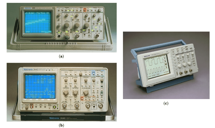
Figure 1: (a) General-purpose oscilloscope; (b) lab-quality oscilloscope; (c) portable oscilloscope (Photos courtesy of Tektronix, Inc.)
In Figure 2a, a “digital storage” oscilloscope (DSO) is shown. In today’s world, you will find these quite commonly used. These scopes have the ability to store signal waveforms in memory for either immediate or later retrieval or display. This type of scope makes possible such applications as waveform comparisons at different times or locations, complex, long-duration and/or short-duration signal change analysis, and other unique types of signal comparisons and analyses. These are analyses that would be difficult or impossible to perform using standard analog real-time (ART) scopes.
The “real-time” identifier simply indicates that what you see on the scope is happening now. To store signals, this scope “digitizes” the analog signals by sampling signal levels many times over the duration of the signal waveform. The digital data is then placed in memory for retrieval at the desired time.
Another generation in scopes, advertised by at least one well-known oscilloscope manufacturer, are those with “automatic measurements” capability, graphical interfaces, saving of image files to storage media disks, connectivity to computers, and other amazing capabilities.
These scopes are advertised as having ability to display, store, and analyze complex signals in real-time, using three dimensions of signal information: amplitude, time, and distribution of amplitude over time. These abilities make this type of scope go beyond analog real-time (ART) and digital storage oscilloscopes’ (DSO) capabilities. See Figure 2b for an example of this type of scope.
Many modern digital oscilloscopes make difficult waveform measurements much easier than was true of the old analog scopes. Front panel buttons and on-screen menus make your selection of automated measurements very intuitive.
Measurements of amplitude, period, rise, or fall times are all easily done. Some of these modern scopes also can perform some mathematics for you in terms of determining mean and RMS calculations, as well as duty cycle computations, and so on. Automated measurements with these scopes appear as on-screen alphanumeric readouts, which are typically more accurate than you could perform by trying to interpret values from the scope graticule.
Also, many modern scopes can produce outputs that can be coupled to computers and printers, which adds further to their flexibility and usefulness.
Two general features that are common to virtually all scopes include the following:
- All scopes have a cathode-ray tube (CRT) where the visual displays are viewed.
- All scopes have controls and related circuits that adjust the display to help you analyze voltage, time, waveform, and frequency parameters of signal(s) under test. In some cases, these controls are manipulated manually; in other cases, they may be automated, depending upon the type of oscilloscope you are using.
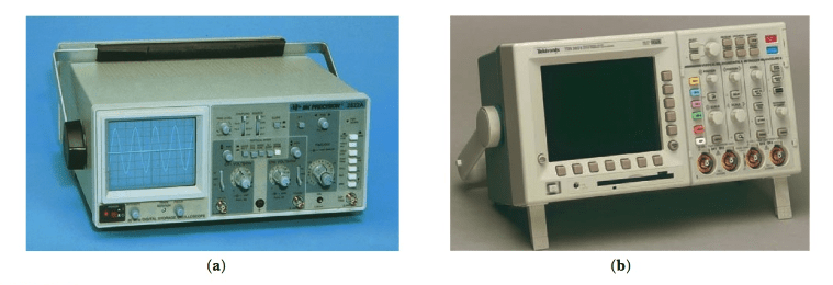
Figure 2: (a) A digital storage oscilloscope (DSO) (Courtesy of B & K Precision); (b) a digital phosphor “high tech” oscilloscope (Courtesy of National Instruments)
Oscilloscope Parts and Function
A simplified sample scope front panel layout is shown in Figure 3. Refer to this figure as you read the following list and descriptions of the various controls and related circuits involved.
The key parts of an oscilloscope that relate to the controls shown in Figure 3 are the following:
The cathode-ray tube (CRT), which consists of a screen where signals are viewed, and the elements within the CRT, which generate and control a stream of electrons that strike the back (inside) of the CRT screen, producing the illumination you view on the outside of the CRT screen. For informational purposes only, note the simplified diagram in Figure 4, showing some of these CRT elements. NOTE: It is not necessary for you to learn details regarding these elements at this time in your training.
Intensity and focus controls, which allow the users to adjust the brightness, size, clarity, and focus of the spot or trace on the CRT screen caused by the electron beam (see Figure 3).
Position controls (vertical and horizontal), which allow adjusting voltages that control the position of the trace on the CRT screen. In Figure 4, you can see the CRT “deflection plates” that control the position and movement of the electron beam coming from the opposite end of the tube and striking the back of the screen.
The position where the electron beam strikes the back of the CRT screen is controlled by the electrostatic field set up between the plates by the difference of potential between them. The reactions of the electron beam to these fields are illustrated in Figure 5. Notice the electron beam is attracted to the plate(s) having a positive charge and repelled from any deflection plates having a negative potential, or charge. Therefore, the position where the electron beam strikes the screen can be controlled by the voltages present at the deflection plates.
Knowing that deflection of the electron beam is toward positive deflection plates and away from negative deflection plates, you can understand the position controls; sim- ply make the appropriate deflection plates either more positive or more negative, de- pending on which way you want the electron beam to move on the CRT face.
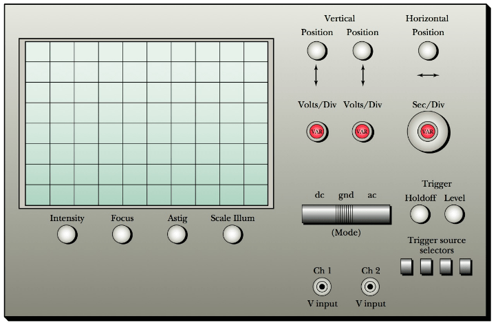
Figure 3: typical controls on a dual-trace scope (simplified)
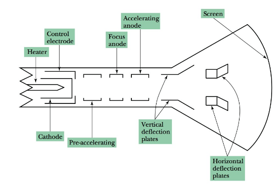
Figure 4: Elements in a typical cathode-ray tube (CRT)
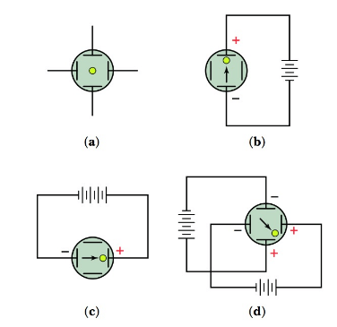
Figure 5: Electron-beam movement caused by dc voltages on deflection plates
Also, observe what happens when an AC signal is applied to the various deflection plates, as shown in Figure 6a, b, and c.
The horizontal sweep frequency controls are used to control the linear trace speed and repetition rate of the horizontal trace of the electron beam across the CRT screen.
A saw-tooth (or ramp-type) waveform applied to the horizontal deflection plates creates a horizontal trace on the screen, Figure 7. The voltage applied to the horizontal plates is sometimes called the horizontal “sweep voltage,” because the voltage causes the electron beam to horizontally sweep across the screen, creating a horizontal trace, or line.
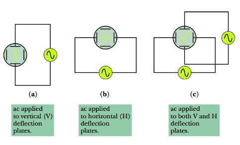
Figure 6: Electron-beam movement caused by ac voltages on deflection plates
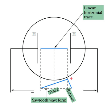
Figure 7: Linear trace caused by saw tooth voltage on horizontal (H) plates
The electron beam moves, or traces at a constant rate (linear speed) across the screen from left to right, then quickly retraces, or “flies back,” to its starting point on the left. During the very short retrace (or fly back) time, a blanking signal is applied to the sys- tem so that the scope screen will not display the electron beam’s movement across the screen (from right to left) during the retrace time.
Because the electron beam is moving at a constant speed across the screen during the left-to-right trace time, a horizontal “time base” has been established. In other words, we know how much time it takes for the beam to move from one horizontal point to another on the screen. Because of this, we can measure times and calculate frequencies of signal waveforms that are displayed, as you will see later.
The number of times the beam traces across the screen in a second is determined by the frequency of the sweep (saw tooth) voltage. You see a horizontal line on the screen when this happens at a rapid rate. Two reasons for this are that:
(1) The CRT screen material has a persistence that causes continual emission of light from the screen for a short time after the electron beam has stopped striking that area; and
(2) The retinas in our eyes also have a persistence feature. This is why you don’t see flicker between frames in movies or on TV.
The sweep frequency controls—horizontal time variable, “VAR,” and horizontal sec/div (seconds per division)-adjust the frequency of the horizontal sweep circuitry in the oscilloscope. This controls the number of times per second the beam is traced horizontally across the CRT screen. The horizontal frequency control(s) allows us to view signals of different frequencies.
Having accumulated this information, let’s now see how the electron beam is further con- trolled, amplified, or attenuated to provide meaningful displays on the CRT screen.
Vertical section is where signals to be analyzed are input into the scope, amplified, or attenuated, as needed for proper viewing. Key elements in this section are the vertical input jack(s) (sometimes called Y input jacks), and the vertical attenuator and vertical amplifier, with related controls. When the scope is a single-trace scope, there is only one vertical input jack. When a dual-trace scope is involved, there are two vertical in- put jacks. (See Chapter 1 and Chapter 2 V input jacks on drawing for Figure 3.)
The vertical attenuator and amplifier circuitry, and associated controls, enable de- creasing or increasing the amplitude of the signals that are applied to the scope via the vertical input jack(s). View Figure 3 again, and note the calibrated vertical volts/div and the variable control(s), which are used to adjust the scopes vertical sensitivity, giving signal level control. Using these controls allows you to adjust for larger or smaller vertical deflection of the CRT trace with a given vertical input signal amplitude.
Horizontal section allows control of voltages and signals applied to the horizontal deflection plates. We have briefly discussed some of the important horizontal deflection elements and controls. One of these controls adjusts the frequency of the internally generated horizontal sweep signal.
Other possible elements related to the horizontal trace may include a horizontal gain control that changes the length of the horizontal trace line, and a jack (often marked “Ext X” input) that enables inputting a signal from an external source to the horizontal deflection system, in lieu of using the internally generated sweep signal.
Synchronization controls are used to synchronize the signal you want to observe with the horizontal trace; thus, the waveform appears stationary (assuming the signal has a periodic waveform). The effect is much like a strobe light that provides “stop action” when timing an automobile, for example. Also, you have probably observed that spinning fan blades can appear to be standing still if the light shining on them is blinking at the appropriate rate.
It is not necessary to go into detail regarding the circuitry, but it is sufficient to say that by starting or “triggering” the trace (left-to-right horizontal sweep) of the electron beam in proper time relationship to the signal to be observed on the scope (signal fed to the vertical deflection plates), a stable waveform is displayed.
Controls and jacks associated with this synchronization process include the following:
- Trigger source selector switches
- “Trigger hold off and level” controls, which help set the appropriate level for the triggering signal to work best. (Again, look at Figure 3 to observe these controls.)
Practical Notes
Caution! One thing you should learn when operating a scope is that it is not good to leave a bright spot at one position on the CRT. The CRT screen material can be burned or damaged if this occurs for any great length of time. Never have the trace bright enough to cause a “halo” effect on the screen.
Oscilloscope Working Principle Key Takeaways
Understanding the components, functions, and types of oscilloscopes is essential for anyone working with electronic signals, as these instruments play a critical role in signal visualization and analysis. From basic analog models to advanced digital storage and high-tech scopes, each type offers unique advantages suited for specific applications—ranging from routine lab diagnostics to complex waveform analysis in research, telecommunications, and embedded systems. Their ability to provide real-time monitoring, automated measurements, data storage, and computer connectivity makes them indispensable tools in electronics testing, troubleshooting, and design.