The article discusses the Node Voltage Method, a systematic technique for analyzing electric circuits by using node voltages as variables. It outlines the step-by-step process for applying this method to both resistive circuits and circuits containing voltage sources, emphasizing the use of Ohm’s Law and Kirchhoff’s Current Law (KCL) to formulate and solve circuit equations.
Node voltage analysis is the most general method for the analysis of electric circuits. Its application to linear resistive circuits is illustrated in this article. The node voltage method is based on defining the voltage at each node as an independent variable. One of the nodes is freely chosen as a reference node (usually—but not necessarily—ground), and each of the other node voltages is relative to this node.
Ohm’s law is used to express resistor currents in terms of node voltages, such that each branch current is expressed in terms of one or more node voltages. Finally, KCL is applied to each non-reference node to generate one equation for each node voltage. The result is that only node voltages and known parameters appear explicitly in the equations.
Figures 1 and 2 illustrate how to apply Ohm’s law and KCL in this method.
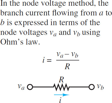
Figure 1 Branch current formulation in node analysis
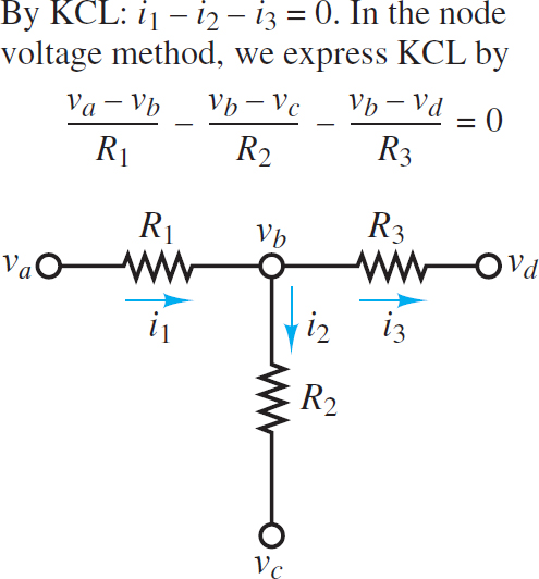
Figure 2 Use of KCL in node analysis
Once each branch current is defined in terms of the node voltages, Kirchhoff’s current law is applied at each node:
$\begin{matrix}\sum i=0 & {} & \left( 1 \right) \\\end{matrix}$
The systematic application of this method to a circuit with n nodes leads to n − 1 equations. However, one node must be chosen as a reference, which is freely and conveniently assigned a value of 0 V. Thus, the result is n − 1 variables (the node voltages) in n − 1 independent linear equations. Node analysis provides the minimum number of equations required to solve the circuit.
Node Analysis Step by Step Guide
1. Select a reference node. Often, the best choice for this node is the one with the most elements attached to it. The voltage associated with each non-reference node will be relative to the reference node, which is (for simplicity) typically assigned a value of 0 V.
2. Define voltage variables ${{v}_{1}},{{v}_{2,\ldots .}}~{{v}_{n-1}}$ for the remaining n − 1 nodes.
• If the circuit contains no voltage sources, then all n − 1 node voltages are treated as independent variables.
• If the circuit contains m voltage sources:
◦There are only (n − 1) − m independent voltage variables.
◦ There are m dependent voltage variables.
◦ For each voltage source, one of the two adjacent node voltage variables (e.g., vj or vk) must be treated as a dependent variable.
3. Apply KCL at each node associated with an independent variable, using Ohm’s law to express each resistor current in terms of the adjacent node voltages. The convention used consistently in this book is that currents entering a node are positive and currents exiting a node are negative; however, the opposite convention could be used.
• For each voltage source there will be one additional dependent equation
(e.g., ${{v}_{k}}=~{{v}_{j}}+~{{v}_{s}}$).
• When a voltage source is adjacent to the reference node, either vj or vk will be the reference node value, which is typically assigned as 0 V, and the additional dependent equation is particularly simple.
4. Collect coefficients for each of the n − 1 variables and solve the linear system of n − 1 equations.
• Some of the dependent equations may have the simple form vk=vs. In this case, the total number of equations and variables is reduced by direct substitution.
This procedure can be used to find a solution for any circuit. A good approach is to first practice solving circuits without any voltage sources and then learn to deal with the added complexity of circuits with voltage sources. The remainder of this section is organized in this fashion.
For some readers, it is advantageous to redraw circuits in an equivalent but non-rectangular manner by viewing the circuit as a collection of circuit elements located between nodes. The right-hand portion of Figure 3 is constructed by first drawing three node circles and then adding in the elements that sit between each pair of nodes. To successfully redraw a circuit or to apply node analysis it is imperative that the correct number of nodes is known. Thus, it is worthwhile to practice recognizing and counting nodes.
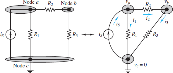
Figure 3 Illustration of node analysis
Details and Examples
Consider the circuit shown in Figure 3. The directions of current i1, i2 and i3 may be selected arbitrarily, however, it is often helpful to select directions that appear to conform with one’s expectations. In this case, is is directed into node a and therefore one might guess that i1 and i2 should be directed out of that same node. Application of KCL at node a yield.
$\begin{matrix}{{i}_{s}}-{{i}_{1}}-{{i}_{2}}=0 & {} & \left( 2 \right) \\\end{matrix}$
Whereas at node b
$\begin{matrix}{{i}_{2}}-{{i}_{3}}=0 & {} & \left( 3 \right) \\\end{matrix}$
It is not necessary nor appropriate to apply KCL at the reference node since that equation is dependent on the other two. It may be useful to demonstrate this fact for this example. The equation obtained by applying KCL at node c is
$\begin{matrix}{{i}_{1}}+{{i}_{3}}-{{i}_{s}}=0 & {} & \left( 4 \right) \\\end{matrix}$
The sum of the equations obtained at nodes a and b yields the same equation. This observation confirms the statement made earlier:
KCL yields n-1 independent equations for a circuit of n nodes. The nth equation is usually chosen to be v=0 for the reference.
When applying the node voltage method, the currents must be expressed in terms of the node voltages. For the example above i1, i2 and i3 can be expressed in terms of va, vb and vc, by applying ohms law. Between nodes a and c the current is:
\[\begin{matrix}{{i}_{1}}=\frac{{{v}_{a}}-{{v}_{c}}}{{{R}_{1}}} & {} & \left( 5 \right) \\\end{matrix}\]
Similarly, for the other two branch currents
\[\begin{matrix}{{i}_{2}}=\frac{{{v}_{a}}-{{v}_{b}}}{{{R}_{2}}} & {} & {} \\{} & {} & \left( 6 \right) \\{{i}_{3}}=\frac{{{v}_{b}}-{{v}_{c}}}{{{R}_{3}}} & {} & {} \\\end{matrix}\]
These expressions for i1, i2, and i3 can be substituted into the two-nodal equation (equations 2 and 3) to obtain:
$\begin{align}& \begin{matrix}{{i}_{s}}-\frac{{{v}_{a}}}{{{R}_{1}}}-\frac{{{v}_{a}}-{{v}_{b}}}{{{R}_{2}}}=0 & {} & \left( 7 \right) \\\end{matrix} \\& \begin{matrix}\frac{{{v}_{a}}-{{v}_{b}}}{{{R}_{2}}}-\frac{{{v}_{b}}}{{{R}_{3}}}=0 & {} & \left( 8 \right) \\\end{matrix} \\\end{align}$
With a little practice, equations 7 and 8 can be obtained by direct observation of the circuit. These equations can be solved for va and vb, assuming that is, R1, R2 and R3 are known. The same equations may be reformulated as follows:
$\begin{matrix}\left( \frac{1}{{{R}_{1}}}+\frac{1}{{{R}_{2}}} \right){{v}_{a}}+\left( -\frac{1}{{{R}_{2}}} \right){{v}_{b}}={{i}_{s}} & {} & {} \\{} & {} & \left( 9 \right) \\\left( -\frac{1}{{{R}_{2}}} \right){{v}_{a}}+\left( \frac{1}{{{R}_{2}}}+\frac{1}{{{R}_{3}}} \right){{v}_{b}}=0 & {} & {} \\\end{matrix}$
Node Analysis with Voltage Sources
In practice, it is quite common to encounter circuits with voltage sources. To illustrate how node analysis is applied to such circuits, consider the circuit in Figure 4. Verify that this circuit has n = 4 total nodes.
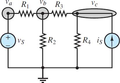
Figure 4 Node analysis with voltage sources
Step 1: Select a reference node. Often, the best choice for this node is the one with the most elements attached to it. The voltage associated with each non-reference node will be relative to the reference node, which is (for simplicity) typically assigned a value of 0 V.
When voltage sources are present, it is also advantageous to pick the reference node so that at least one of those voltage sources is attached to it. In Figure 5, the reference node, denoted by the ground symbol, is assumed to have a value of 0 V.

Figure 5 Node analysis with voltage sources
Step 2: Label the remaining n − 1 nodes with voltage variables ${{v}_{1}},{{v}_{2,\ldots .}}~{{v}_{n-1}}$ If the circuit contains m voltage sources:
• There are only (n − 1) − m independent voltage variables.
• There are m dependent voltage variables.
• For each voltage source, one of the two adjacent node voltage variables (e.g.,vj or vk) must be treated as a dependent variable.
The remaining three (4 − 1 = 3) node voltages are labeled va and vb, and vc as shown in Figure 5. Since the circuit contains one (m = 1) voltage source, there are two (4−1−1 = 2) independent variables and one dependent variable. The only va is adjacent to the voltage source; thus, it is the one dependent variable.
Apply KCL at each node associated with an independent variable, using Ohm’s law to express each resistor current in terms of the adjacent node voltages. Currents entering a node are assumed to be positive while those exiting a node are assumed to be negative.
• For each voltage source Vs there will be one additional dependent equation (e.g., Vk = vj + Vs).
• When a voltage source is adjacent to the reference node, either vj or vk, will be the reference node value, which is typically assigned as 0 V, and the additional dependent equation is particularly simple.
Apply KCL at the two nodes associated with the independent variables vb and vc:
At node b:
$\begin{matrix}\frac{{{v}_{a}}-{{v}_{b}}}{{{R}_{1}}}-\frac{{{v}_{b}}-0}{{{R}_{2}}}-\frac{{{v}_{b}}-{{v}_{c}}}{{{R}_{3}}}=0 & {} & \left( 10a \right) \\\end{matrix}$
At node c:
$\begin{matrix}\frac{{{v}_{b}}-{{v}_{c}}}{{{R}_{3}}}-\frac{{{v}_{c}}}{{{R}_{4}}}+{{i}_{s}}=0 & {} & (10b) \\\end{matrix}$
The equation for the dependent variable Va is simply:
$\begin{matrix}{{v}_{a}}=0+{{v}_{s}}={{v}_{s}} & {} & (10c) \\\end{matrix}$
Step 4: Collect coefficients for each of the n − 1 variables, and solve the linear
system of n − 1 equations.
• Some of the dependent equations may have the simple form vk = vs. In this case, the total number of equations and variables is reduced by direct substitution.
Substitute for va in equation 10a. At node b:
$\begin{matrix}\frac{{{v}_{s}}-{{v}_{b}}}{{{R}_{1}}}-\frac{{{v}_{b}}}{{{R}_{2}}}-\frac{{{v}_{b}}-{{v}_{c}}}{{{R}_{3}}}=0 & {} & \left( 11 \right) \\\end{matrix}$
Finally, collect the coefficients of the two independent variables to express the system of two equations as:
$\begin{matrix}\left( \frac{1}{{{R}_{1}}}+\frac{1}{{{R}_{2}}}+\frac{1}{{{R}_{3}}} \right){{v}_{b}}+\left( -\frac{1}{{{R}_{3}}} \right){{v}_{c}}=\frac{1}{{{R}_{1}}}{{v}_{s}} & {} & {} \\{} & {} & \left( 12 \right) \\\left( -\frac{1}{{{R}_{3}}} \right){{v}_{b}}+\left( \frac{1}{{{R}_{3}}}+\frac{1}{{{R}_{4}}} \right){{v}_{c}}={{i}_{s}} & {} & {} \\\end{matrix}$
The resulting system of two equations in two unknowns is now ready to be solved.
Node Voltage Method Key Takeaways
The Node Voltage Method is a foundational technique in circuit analysis, offering a systematic and efficient approach for solving both simple and complex electrical networks. Its importance lies in its ability to reduce the number of equations needed to analyze a circuit, especially in large systems with many components. By focusing on node voltages as the primary variables and applying Kirchhoff’s Current Law (KCL) alongside Ohm’s Law, engineers can derive accurate solutions using linear algebraic methods. This technique is particularly valuable in applications such as circuit simulation, integrated circuit design, and power system analysis, where efficiency, scalability, and accuracy are critical.