The article introduces the concept of Fourier series as a method for analyzing periodic signals by expressing them as a sum of sinusoidal components. It discusses various representations of Fourier series, the computation of their coefficients, and their application in modeling signal responses in linear systems.
The aim of this article is to introduce the concept of frequency domain analysis of signals, and specifically the Fourier series. Later in this article, we explain how it is possible to represent periodic signals by means of the superposition of various sinusoidal signals of different amplitude, phase, and frequency. Let the signal x(t) be periodic with period T, that is,
\[\begin{matrix}x(t)=x(t+T)=x(t+nT) & n=1,2,3,…..;T=period & \begin{matrix}{} & (1) \\\end{matrix} \\\end{matrix}\]
An example of a periodic signal is shown in Figure 1.
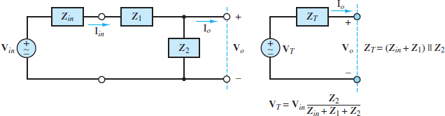
Figure 1 Thevenin equivalent source network
The signal x (t) can be expressed as an infinite summation of sinusoidal components, known as a Fourier series, using either of the following two representations.
Fourier Series:
- Sine-cosine (quadrature) representation
\[x(t)={{a}_{0}}+\sum\limits_{n=1}^{\infty }{{{a}_{n}}\cos \left( n\frac{2\pi }{T}t \right)+\sum\limits_{n=1}^{\infty }{{{b}_{n}}\sin \left( n\frac{2\pi }{T}t \right)}}\begin{matrix}{} & (2) \\\end{matrix}\]
- Magnitude and phase form
\[x(t)={{c}_{0}}+\sum\limits_{n=1}^{\infty }{{{c}_{n}}}\sin \left( n\frac{2\pi }{T}t+{{\theta }_{n}} \right)\begin{matrix}{} & (3) \\\end{matrix}\]
\[x(t)={{c}_{0}}+\sum\limits_{n=1}^{\infty }{{{c}_{n}}\cos \left( n\frac{2\pi }{T}t-{{\psi }_{n}} \right)}\begin{matrix}{} & (4) \\\end{matrix}\]
In each of these expressions, the period T is related to the fundamental frequency of the signal ωo by
\[{{\omega }_{0}}=2\pi {{f}_{0}}=\frac{2\pi }{T}\begin{matrix}{} & rad/s\begin{matrix}{} & (5) \\\end{matrix} \\\end{matrix}\]
The frequencies 2ωo, 3ωo, 4ωo, etc., are called harmonics.
It is straightforward to show that equations 2 and 3 are equivalent when the parameters an, bn, cn and 𝜃n are defined by:
\[\begin{matrix}\sqrt{{{a}_{n}}^{2}+{{b}_{n}}^{2}}={{c}_{n}} & and & \frac{{{b}_{n}}}{{{a}_{n}}}=\cot \left( {{\theta }_{n}} \right) & (6) \\\end{matrix}\]
Similarly, one can show that equations 2 and 4 are equivalent when the parameters an, bn, cn, and 𝜃n are defined by:
\[\begin{matrix}\sqrt{{{a}_{n}}^{2}+{{b}_{n}}^{2}}={{c}_{n}} & and & \frac{{{b}_{n}}}{{{a}_{n}}}=\tan \left( {{\psi }_{n}} \right) & (7) \\\end{matrix}\]
Figure 2 is a graphical representation of the equivalence of the {an, bn} and {cn , 𝜃n} forms of the Fourier series.
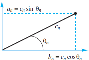
Figure 2 Relationship between {an , bn} and {cn , 𝜃n} forms
Each of the two forms of the Fourier series, equations 2 and 2 (or 4), has its distinct advantages. The sine-cosine representation uses odd and even functions of the independent variable. Odd functions are anti-symmetric about the origin and satisfy the condition:
\[f(-t)=-f(t)\begin{matrix}{} & odd\begin{matrix}function\begin{matrix}{} & (8) \\\end{matrix} \\\end{matrix} \\\end{matrix}\]
Sine functions are odd. Even functions are symmetric about the origin and satisfy the condition:
\[f(-t)=f(t)\begin{matrix}{} & even\begin{matrix}function\begin{matrix}{} & (9) \\\end{matrix} \\\end{matrix} \\\end{matrix}\]
Cosine functions are even, as is any constant, such as a0. Figure 3 shows even and odd function examples.
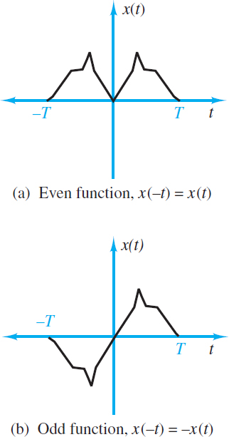
Figure 3 Definition of even and odd functions
The advantage of the representation is that if x(t) is known to be odd (even), it can be represented as the sum of only odd (even) functions [i.e., using only the sine (cosine) terms], thus resulting in easier evaluation of the Fourier series coefficients.
The magnitude and phase forms separate out the magnitude information cn from the phase information 𝜃n or ψn. In this form, Fourier series may be combined readily with magnitude and phase representations of linear systems to periodic inputs. The magnitude and phase components are often represented as a discrete frequency spectrum, as shown in Figure 4.
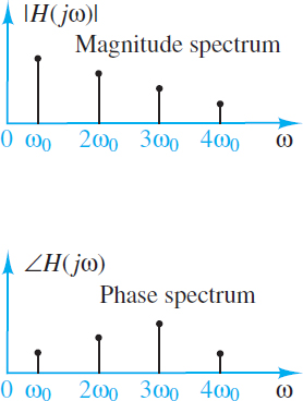
Figure 4 Discrete frequency spectrum
Computation of Fourier Series Coefficients
The computation of the {an, bn} and {cn , 𝜃n} coefficients for the periodic function x (t) is based on the following formulas:
\[\begin{matrix}{{a}_{0}}=\frac{1}{T}\int\limits_{0}^{T}{x(t)dt}=\frac{1}{T}\int\limits_{-T/2}^{T/2}{x(t)dt} & \text{average value of x(t)} & (9) \\\end{matrix}\]\[\begin{matrix}{{a}_{n}}=\frac{2}{T}\int\limits_{0}^{T}{x(t)\cos \left( n\frac{2\pi }{T}t \right)}dt=\frac{2}{T}\int\limits_{-T/2}^{T/2}{x(t)\cos \left( n\frac{2\pi }{T}t \right)dt} & {} & (10) \\\end{matrix}\]
\[\begin{matrix}{{b}_{n}}=\frac{2}{T}\int\limits_{0}^{T}{x(t)\sin \left( n\frac{2\pi }{T}t \right)}dt=\frac{2}{T}\int\limits_{-T/2}^{T/2}{x(t)\sin \left( n\frac{2\pi }{T}t \right)dt} & {} & (11) \\\end{matrix}\]
The integral limits are written in two different forms to illustrate that it does not matter where the integration starts, provided that it is carried out over one entire period. The cn and 𝜃n (or ψn) values can be derived from the an and bn coefficients.
To illustrate the significance of the Fourier series decomposition, consider the square wave of Figure 5(a), which is an even function. Only even function (cosine) terms are non-zero. The first six non-zero Fourier series terms are shown in Figure 5(b).
Note that the first term corresponds to ao, which is the average value A/2 of the function. The other five terms correspond to n odd (1, 3, 5, 7, and 9). Note also that the coefficients for n = 1, 5, and 9 are positive, and those for n = 3 and 7 are negative (you can see this by looking at the peaks of the cosine waveforms). This alternation of positive and negative cosines is required so that each term can add or subtract from the previous terms as needed to “latten” the waveform into a square wave.
Figure 5(c) compares the original square wave with the Fourier series approximation. It should be evident that 10 terms are not sufficient to reproduce the sharp edges of the square wave, but it should also be clear that as we add more Fourier terms, the resulting approximation will be closer and closer to the square wave signal.
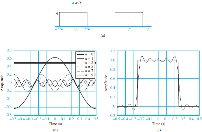
Figure 5 Square wave and its representation by a Fourier series. (a) Square wave (even function); (b) first six Fourier’s series terms of square ware; (c) sum of first six Fourier series terms superimposed upon a square wave
The complete Fourier series for the square wave shown in Figure 5(a) is:
\[f(t)=\frac{A}{2}+\frac{2A}{\pi }\sum\limits_{n=1}^{\infty }{{{(-1)}^{(n-1)}}\frac{\cos \left[ \left( 2n-1 \right)\left( 2\pi \right)t/T \right]}{2n-1}}\]
It is interesting to note that if the square wave shown in Figure 5(a) were shifted to the right by T/4 the resulting waveform would be an odd function. For such a square wave, its value over the interval 0 < t < T /2 is A while its value over the interval T /2 < t < T is zero. The complete Fourier series now contains only odd functions (sines) and is:
\[f(t)=\frac{A}{2}+\frac{2A}{\pi }\sum\limits_{n=1}^{\infty }{\frac{\sin \left[ \left( 2n-1 \right)\left( 2\pi \right)t/T \right]}{2n-1}}\]
The Fourier series for a few other common waveforms are listed below. In each case the peak-to-trough amplitude is A, the period is T, and the average value is A/2.
\[f(t)=\frac{A}{2}+\frac{A}{\pi }\sum\limits_{n=1}^{\infty }{\frac{\sin \left[ \left( 2n\pi t/T \right) \right]}{n}}\begin{matrix}{} & \begin{matrix}Sawtooth\begin{matrix}wave \\\end{matrix} \\\end{matrix} \\\end{matrix}\]
\[f(t)=\frac{A}{2}-\frac{4A}{{{\pi }^{2}}}\sum\limits_{n=1}^{\infty }{\frac{\cos \left[ \left( 2n-1 \right)\left( 2\pi \right)t/T \right]}{{{(2n-1)}^{2}}}}\begin{matrix}{} & Triangle\text{ }\begin{matrix}wave \\\end{matrix} \\\end{matrix}\]
These Fourier series converge everywhere that the function itself is differentiable. The Fourier series for the square wave does not converge at t = 0, T /2, T . . . while the Fourier series for the sawtooth wave does not converge at t = 0, T, 2T…
Response of Linear Systems to Periodic Inputs
The frequency response concept is particularly useful when one deals with a system excited by a periodic input, which can be modeled by a Fourier series of sinusoids of known amplitude and phase, but different frequencies. Assume that the Fourier series has a finite number of terms:
\[x(t)={{c}_{0}}+\sum\limits_{n=1}^{N}{{{c}_{n}}\sin \left( n\frac{2\pi }{T}t+{{\theta }_{n}} \right)}\begin{matrix}{} & (12) \\\end{matrix}\]
Each of the N sinusoids is characterized by amplitude cn, phase 𝜃n, and frequency ωn = nωo, where ωo = 2π/T and T is the period of the input signal. For example, the periodic input could be the sawtooth waveform.
Figure 6 illustrates the input-output representation of a system, making use of the frequency response concept.
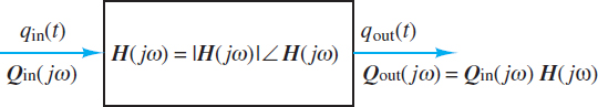
Figure 6 Response of a linear system to a phasor input
The figure shows that if the input qin (t) to a linear system can be represented by the phasor Qin (jω), then output can be computed by multiplying the phasor input by the frequency response function of the linear system. This product is a complex number that can be computed by multiplying the magnitude of the input phasor by the magnitude of the frequency response function and by adding the phase angle of the input phasor to the phase angle of the frequency response.
In the case of a periodic input expressed in terms of a (truncated) Fourier series, we must recognize that each of the input sinusoidal components propagates through the system according to the frequency response. Thus, the discrete magnitude spectrum of the periodic output signal in the steady state is equal to the discrete magnitude spectrum of the input signal multiplied by the amplitude ratio of the frequency response of the system at the appropriate frequencies.
The phase spectrum of the output signal in the steady state is equal to the phase spectrum of the input signal added to the phase angle frequency response of the system at the appropriate frequencies.
If x(t) is the input to a linear system in the form given, and if the linear system has a frequency response function H( jω), then the output of the system y(t) is given by
\[y(t)=\sum\limits_{n=1}^{N}{\left. \left| H \left( j{{\omega }_{n}} \right) \right. \right|}{{\begin{matrix} c \\\end{matrix}}_{n}}\sin \left[ {{\omega }_{n}}t+{{\theta }_{n}}+\angle H \left( j{{\omega }_{n}} \right) \right]\begin{matrix} {} & (13) \\\end{matrix}\]
Where |H(jωn)| and ∠H(jωn) are the magnitude and phase, respectively, at the frequency corresponding to the nth harmonic nωo of the input.
Fourier series Key Takeaways
The Fourier series plays a fundamental role in understanding and analyzing periodic signals by breaking them down into sums of simple sinusoidal components. This decomposition not only simplifies the study of signals but also makes it easier to predict and model the behavior of linear systems in response to periodic inputs. The ability to separate a signal into magnitude and phase components is especially valuable in fields like communications, signal processing, and electrical engineering, where analyzing the frequency spectrum is crucial for system design and performance optimization. Whether in reconstructing complex waveforms such as square or triangle waves, or in analyzing real-world signals, the Fourier series serves as a powerful tool for engineers and scientists to work effectively in the frequency domain.