The article provides a comprehensive overview of residential photovoltaic (PV) system design, focusing on key considerations such as system configuration (grid-connected vs. stand-alone), load and solar resource evaluation, technology selection, array sizing, and inverter matching. It highlights the impact of physical, financial, and environmental factors on PV system performance and design efficiency.
The task of designing Photovoltaic (PV) systems is a very tricky process due to the fact that PV panels are still relatively expensive and energy production is very sensitive to atmospheric conditions and the physical location.
In the case of ground-mounted PV systems, one can choose the optimum tilt angle and orientation, and often the physical size is the only limiting factor.
In the case of residential PV systems, PV panels are usually mounted on the roof, which might not have the optimum angle or orientation. Besides these limitations, the size of the roof is fixed; therefore, several parameters are already fixed at the beginning of the design.
Such design parameters or constraints will affect the following:
- The required annual energy production (AEP)
- The available budget for the installation
- Location-specific limitations: roof size, tilt, and orientation
The first task is to decide whether the PV system will be connected to the electrical grid.
Afterward, the load pattern should be evaluated in order to estimate power and energy requirements. When these requirements have been defined, the PV cell technology can be chosen; the PV array can be sized for the required amount of power.
Furthermore, the PV array needs to be configured to fit the specifications of the PV inverter. Finally, at the end of this chapter, the whole design procedure is evaluated through a case study, by using freely available design tools. The results are presented and discussed.
Grid-Connected or Stand-Alone Systems
Residential PV systems can be divided into two major groups: grid-connected or stand-alone.
A PV system can be connected to the electrical grid when the house is connected to the low-voltage (LV) utility network; thus, the power network can be used to dump the surplus energy production.
The PV system can be connected to the energy meter of the house, thereby increasing self-consumption. Another solution is to add an individual energy meter that measures the energy that the PV system produces, which is then accounted for separately.
Both energy metering solutions are presented in Figure 1.
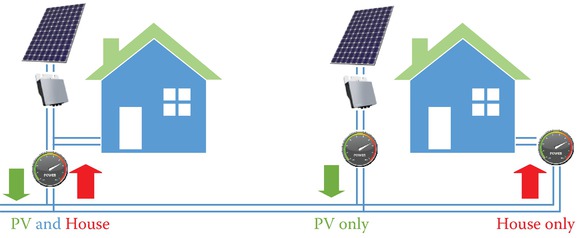
Figure 1 Energy metering of a residential grid-connected PV system, which can be connected to the same energy meter or have a separate meter for measuring PV production.
In both cases, the grid is used like a large battery, storing the surplus energy produced by the PV system. Thus, in such a case, during periods with high irradiation and low load conditions, the grid will be stressed, leading to voltage rise, due to the mainly resistive nature of the LV network.
To mitigate the problem of voltage rise, PV inverters are nowadays required to support the grid with reactive power, thereby keeping the grid voltage within the limits imposed by the grid codes.
On the other hand, in houses in remote areas that are far away from any electrical network, a stand-alone PV system has to be installed.
The complexity of the design will increase since one can install a battery pack to store the produced energy, which can be used later when extra energy is required. In this case, an extra converter is needed, which controls the state of charge of the battery and communicates this information to the PV system control.
To increase the penetration of PV and the self-consumption ratio, advanced storage solutions using Li-ion batteries can also be added to grid-connected PV systems. This trend can mainly be observed in Germany and Japan, where self-consumption is encouraged and has been subsidized since 2013.
Up until now, more than 15,000 German households use PV systems that are combined with battery storage.
Load Pattern Evaluation (Cover the Load over 1-Hour/1-Year Periods)
In the case of residential homes, the average load profile shows two distinct peaks during the morning and evening hours, while it is much lower with a flat shape during the working hours on weekdays, as detailed in Figure 2.
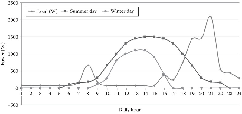
Figure 2 Typical residential load profile compared to the production of a 1.5 kWp PV system on a summer day and on a winter day on the Northern Hemisphere.
Such a load profile does not match the PV energy production curves, which are shown with dotted lines in the above figure.
During a sunny day, production starts at sunrise, gradually increasing with the available sunshine, and peaks around noon, gradually decreasing as a function of irradiation until sundown.
This means that there are periods during the day when the power flows toward the grid (also called as reverse power flow in the literature) and the house becomes a negative load, while during peak load periods, the energy is supplied from the grid again.
Therefore, it is important to decide how much power and energy the designed PV system needs to cover, on a daily, monthly, or even yearly period.
Solar Resource Evaluation
The available sunshine hours will have a direct influence on the payback time of the designed PV system.
In southern Europe, the payback time is around 5–6 years, while in central and northern Europe, the payback time can reach periods up to 9–10 years or even longer, depending on the local energy price.
This means that the PV system will produce the energy for “free” only after these years have passed.
If the location for the PV system is known, then there are several free tools online, for example, PVGIS (http://re.jrc.ec.europa.eu/pvgis/apps4/pvest.php) that use the average irradiation data from satellite images of the last 10 years.
Based on this, the monthly and yearly energy production data in kWh/m2/year/kWp for the chosen location, both for horizontal and for the optimum tilt angle, can be predicted, as shown in Figure 3.

Figure 3 Estimated monthly energy production in kWh for a 1 kWp PV system at an optimum tilt in Aalborg (Denmark) and Bari (Italy).
The physical placement of the panels is also of importance. If the location is known, then a Sun chart can be plotted, where the elevation (position of the sun) is given for the whole year.
Furthermore, if the height and distance to shading sources (trees, neighboring houses) are known, this information can also be added to the Sun chart, as shown with a black dashed line in Figure 4.
Based on this, the periods when shadows will be cast over the PV system and the extent of their influence on the energy production can be estimated. Such a shaded period can be seen in the below picture, where some trees have been considered as sources of shadow.
As a consequence, on December 21 and January 21, the PV panels are permanently under shadow before noon.
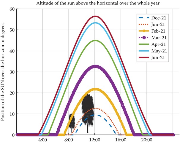
Figure 4 Sun chart for Aalborg location (latitude, 57; longitude, 9.5) showing also sources of shading during certain periods of the year represented by two trees.
PV Array Sizing (kWp) (Over- versus under sizing)
With a good estimation of the required AEP and the data for the available kWh/m2/year/kWp, one can roughly estimate the size of the PV array for the different PV technologies.
It is important to mention that the different technologies have different cell efficiencies and price. Therefore, the cost, physical size, and AEP of the designed PV system will be influenced by the chosen PV cell technology.
There are three main technologies within the market today:
- Monocrystalline silicon PV cells, which have the highest efficiency, but are the most expensive
- Multi-crystalline silicon PV cells, which offer a trade-off between efficiency and price
- Thin-film (TF) PV cells, which tend to have the lowest efficiency, although price/m2 might be the lowest
Depending on the design parameters, one can choose the technology that best fits the constraints. In this way, the PV system can be optimized for minimum investment cost or maximum energy production.
Table 1 presents a comparison of the different PV cell technologies, based on panel efficiency and required surface for a power level of 1 kWp.
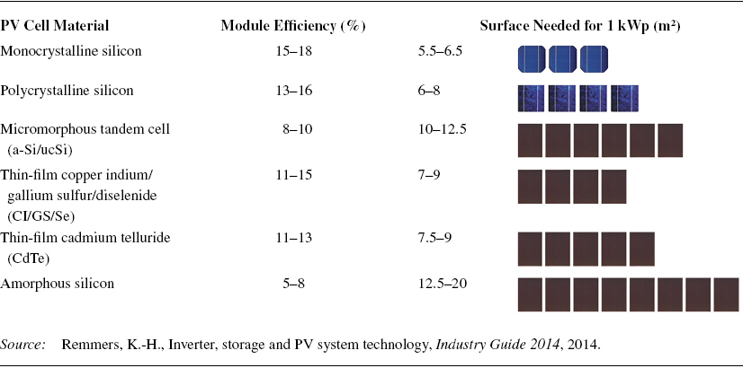
TABLE 1 Efficiency of Different PV Cell Technologies
Choosing the String and Array Configuration
Now that the solar cell technology and the kWp size for the PV array have been chosen, one will need to connect the individual PV panels into strings and arrays in order to achieve a certain maximum power point (MPP) voltage and current rating at standard test conditions (STC).
STC is defined as 1000 W/m2 irradiance intensity, 25 °C cell temperature and an irradiance spectrum corresponding to an air mass ratio of 1.5; PV panel datasheet values are universally given in STC.
It is always recommended to recalculate the MPP voltage and current for extreme conditions for the PV panel temperature. For winter, this temperature is considered to be −10 °C while for summer it is +40 °C.
Knowing the MPP voltage and current range during all conditions, one will be able to find a suitable PV inverter.
Choosing the PV Inverter
A PV inverter will convert the DC current supplied by the PV panels into a grid-synchronized AC current that can be injected into the distribution network.
Commercial PV inverters will make sure that the injected energy satisfies the grid codes and standards enforced by the distribution system operator.
PV inverters work with a wide range of power levels in a day. This is due to the fact that a PV array will deliver its kWp rating only during high irradiation conditions.
When the cell temperature increases or the irradiation decreases, the delivered power by the array drops as well. This is why the efficiency of PV inverters is expressed using a weighted formula that is adjusted to the specific location scenario:
\[{\eta _{EU}} = 0.03{\eta _{5\% }} + 0.06{\eta _{10\% }} + 0.13{\eta _{20\% }} + 0.1{\eta _{30\% }} + {0.48_{\eta 50\% }} + 0.2{\eta _{100\% }}\]
\[{\eta _{CEC}} = 0.04{\eta _{10\% }} + 0.05{\eta _{20\% }} + 0.12{\eta _{30\% }} + 0.21{\eta _{50\% }} + 0.53{\eta _{75\% }} + 0.05{\eta _{100\% }}\]
Where
ηEU is the European weighted efficiency, tailored for locations in central and northern Europe
ηCEC is the Californian efficiency, for locations with a lot of sunshine hours, like California and southern Europe
PV inverters are designed to achieve the highest possible efficiency over a wide power range, nevertheless, only at an optimum voltage range. This can be seen in Figure 5, which details the test measurements of a commercial PV inverter.
The highest efficiency curve is achieved at 600 V input voltage over the whole power range of the inverter.
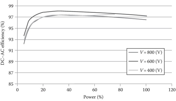
Figure 5 PV inverter efficiency at different input voltages and power levels.
It is important to configure the PV array in such a way that best fits the PV inverter efficiency curve, MPP voltage range, and maximum allowable DC-link voltage, thereby eliminating any type of unnecessary losses and limitations and maximizing the AEP for the designed PV system.
As an example, a PV panel is chosen, for example, the RPP250 UP72 from REW Solartechnik with the datasheet values given in Table 2.
Using the datasheet values of the chosen PV panel, a string can be configured. Such a string design case has a minimum of 8 panels in series and a maximum of 16.
In this way, the PV string parameters can be calculated based on the datasheet values from Table 2.

TABLE 2 Datasheet Values for the Chosen PV Panel
Comparing the PV array configuration from Table 3 to the datasheet values of the PV inverter shown in Table 4, the sizing of the array and the choice of PV inverter can be obtained.
This is an iterative process that should result in an optimum solution with the best match between the electrical specification for the PV array and the PV inverter.
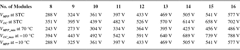
TABLE 3 PV String Configuration for Different Number of Panels Connected in Series
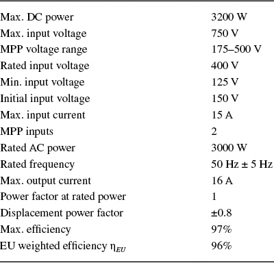
TABLE 4 Datasheet Values for the Chosen PV Inverter
In certain cases, the initial sizing of the PV array will lead to voltage and/or current ranges that will not fit the limits of the maximum power point tracker (MPPT) or the specifications of the PV inverter.
For example, the maximum power point (MPP) voltage could be outside the range of the PV inverter specifications. In such a case, the MPPT algorithm of the PV inverter will limit the output power according to the allowable voltage range. This means that the PV system will not operate at its maximum capability, resulting in a reduced AEP.
Therefore, in such cases, it is recommended to configure a new PV array or choose another PV inverter that better fits the electrical parameters of the initial configuration of the PV array.
What Is the Yield and Performance Ratio?
Finally, the PV system has been designed and configured for delivering the maximum energy in optimum conditions.
To estimate the monthly and yearly energy production, a simple simulation model can be built, where all the components are modeled and real-life data are used for irradiation, cell temperature, availability of grid, etc.
Usually, 1-minute averaged data are used for such simulations, but in certain cases, 1-second averaged data are recommended, to show a realistic scenario also for locations with fast-changing atmospheric conditions (fast cloud movements).
In certain cases, it can happen that when data with a lower resolution are used, the peak irradiation values are filtered out and the converter is sized based on these averaged irradiation values, resulting in power limitations during high-irradiation periods and thereby resulting in energy loss.
Such a scenario is shown in Figure 6, which presents sampled data with 5-minute averaged values in Figure 6a and data with 1-hour averaged values in Figure 6b, for a 48-hour period.
PV systems vary based on the location, PV technology, kWp size, PV array configuration, and also PV inverter type, just to mention a few. This means that direct power production or energy yield will not lead to the best criteria for comparing the performance of different PV systems.
A simple way to measure the performance of a PV system is to compare the measured yearly energy yield to the same PV system under ideal conditions. The influence of the array size can be eliminated in case the produced energy is divided by the nominal power of the PV system at STC.
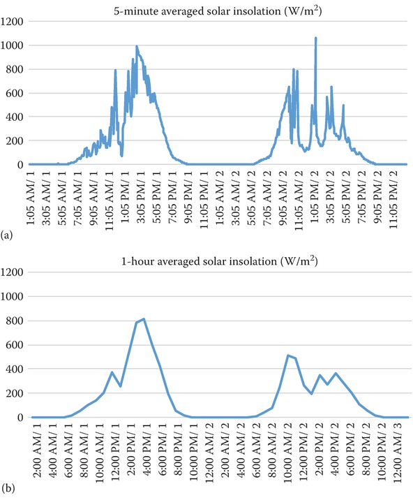
Figure 6 The same measured irradiation data for a 48-hour period in the same location, presented with different averaging periods: 5-minute averaged values (a) and 1-hour averaged values (b).
Using this idea, several performance factors can be defined.
Final yield:
\[{{Y}_{F}}=\frac{{{E}_{usable}}}{{{P}_{G0}}}\]
Where
Eusable is the net energy output of the PV system
PG0 is the nominal power of the PV system at STC
The final yield includes all losses up to the point of connection to the AC electrical network.
Array yield:
\[{{Y}_{A}}=\frac{{{E}_{A}}}{{{P}_{G0}}}\]
Where
EA is the DC energy of the PV system
PG0 is the nominal power of the PV system at STC
The array yield only takes into account the losses up to the DC side of the PV inverter.
Reference yield:
\[{{Y}_{R}}=\frac{{{H}_{G}}}{{{G}_{0}}}=\frac{{{H}_{G}}}{{{G}_{STC}}}\]
Where
HG is the total insolation over the predefined period
GSTC is the insolation at STC: 1000W/m2; 25°C; AM 1.5
Using such performance indicators, it is possible to estimate the different losses, presented in Figure 7, occurring over the whole energy transfer chain of the PV system.
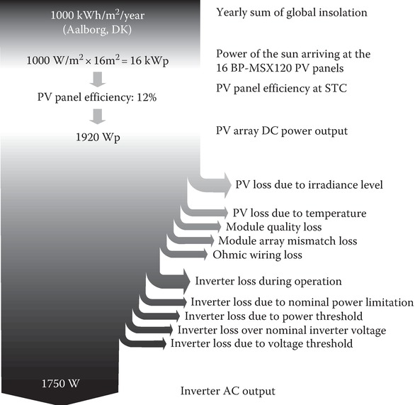
Figure 7 PV system losses, including all the sources for loss throughout the whole energy conversion chain, starting from the available energy from the solar insolation up till the point of connection to the distribution network of the AC grid.
These losses could be generator losses, defined as
\[{{L}_{C}}={{Y}_{R}}-{{Y}_{A}}={{L}_{CT}}+{{L}_{CM}}\]
Where
\[{{L}_{CT}}={{P}_{G0}}[1+{{c}_{T}}({{T}_{C}}-{{T}_{STC}})]\]
Where
cT is the thermal coefficient for power
TC is the cell temperature
TSTC is the temperature at STC
LCM represents non-temperature related losses (miscellaneous capture losses)
That are due to
- String diodes and wiring
- Partial shading, dust, and snow on the panels
- Module mismatch
- PV inverter tracking errors (MPPT)
- Errors in irradiation measurement
There are also considered system losses that are defined as
\[{{L}_{BOS}}={{Y}_{A}}-{{Y}_{F}}\]
Which includes the total losses without the generator losses, like in the case of DC–AC conversion.
Now that all these yields and losses have been defined; the final performance indicator can be defined, which has been named as performance ratio (PR):
\[{{P}_{R}}=\frac{{{Y}_{F}}}{{{Y}_{R}}}\]
Giving a value of the degree for approximation to the ideal case. Using this performance indicator, the performances of PV systems of different sizes, PV cell technologies, and PV inverters and located in different corners of the world can be compared.
Residential Photovoltaic (PV) System Design Key Takeaways
The design considerations discussed in this article are essential not only for optimizing the performance and efficiency of residential photovoltaic (PV) systems but also for ensuring their practical viability and economic feasibility. Each design element—from choosing between grid-connected or stand-alone systems, evaluating load patterns, and assessing solar resources, to selecting the appropriate PV technology and inverter—plays a critical role in meeting energy demands effectively while minimizing costs and environmental impact. These aspects are crucial in real-world applications where space, budget, and energy needs are constrained. A well-designed PV system maximizes energy yield, improves return on investment, and contributes to sustainable energy goals.