The article provides an overview of power calculations in AC circuits, focusing on instantaneous and average power, root mean square (rms) values, impedance and power triangles, and the significance of power factor. It explains how sinusoidal voltages and currents interact in linear circuits and how phase relationships influence real power dissipation.
When a linear electric circuit is excited by a sinusoidal source, all voltages and currents in the circuit are also sinusoids of the same frequency as the source. Figure 1 depicts the general form of a linear AC circuit.
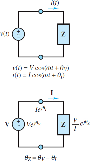
Figure 1 Time and frequency domain representations of an AC circuit. The phase angle of the load is θZ = θV − θI.
The most general expressions for the voltage and current delivered to an arbitrary load are as follows:
\[\begin{matrix}\begin{align}& v(t)=V\cos (\omega t+{{\theta }_{V}}) \\& i(t)=I\cos (\omega t+{{\theta }_{I}}) \\\end{align} & {} & (1) \\\end{matrix}\]
Where V and I are the peak amplitudes of the sinusoidal voltage and current, respectively, and θV and θI are their phase angles. Two such waveforms are plotted in Figure 2, with unit amplitude, angular frequency 150 rad/s, and phase angles θV = 0 and θI = π/3.
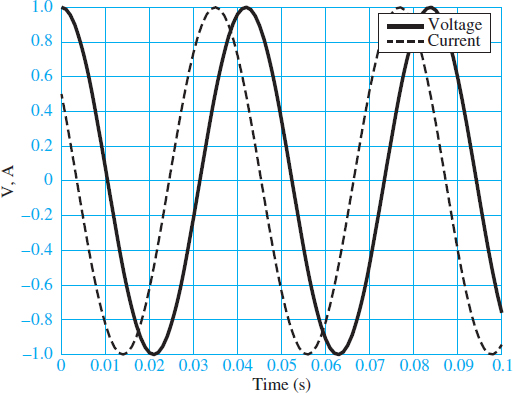
Figure 2 Current and voltage waveforms with unit amplitude and a phase shift of 60°.
Notice that the current leads the voltage; or equivalently, the voltage lags the current. Keep in mind that all phase angles are relative to some reference, which is usually chosen to be the phase angle of a source. The reference phase angle is freely chosen and therefore usually set to zero for simplicity. Also keep in mind that a phase angle represents a time delay of one sinusoid relative to its reference sinusoid.
The instantaneous power dissipated by any element is the product of its instantaneous voltage and current.
\[\begin{matrix}p(t)=v(t)i(t)=VI\cos (\omega t+{{\theta }_{V}})\cos (\omega t+{{\theta }_{I}}) & {} & (2) \\\end{matrix}\]
This expression is further simplified with the aid of the trigonometric identity:
\[\begin{matrix}2\cos (x)cos(y)=\cos (x+y)+\cos (x-y) & {} & (3) \\\end{matrix}\]
Let x=ωt + θV and y=ωt + θI to yield:
\[\begin{matrix}\begin{align}& p(t)=\frac{VI}{2}[\cos (2\omega t+{{\theta }_{V}}+{{\theta }_{I}})+\cos ({{\theta }_{V}}-{{\theta }_{I}})] \\& =\frac{VI}{2}[\cos (2\omega t+{{\theta }_{V}}+{{\theta }_{I}})+\cos ({{\theta }_{Z}})] \\\end{align} & {} & \left( 4 \right) \\\end{matrix}\]
Equation 4 illustrates that the total instantaneous power dissipated by an element is equal to the sum of a constant $\frac{1}{2}$VI cos (θZ) and a sinusoidal $\frac{1}{2}$ VI cos (2ωt + θV + θI), which oscillates at twice the frequency of the source. Since the time average of a sinusoid is zero over one period or over a sufficiently long interval, the constant $\frac{1}{2}$VI cos (θZ) is the time averaged power dissipated by a complex load Z, where θZ is the phase angle of that load.
Figure 3 shows the instantaneous and average power corresponding to the voltage and current signals of Figure 2.
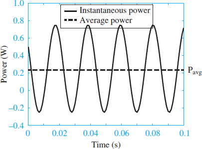
Figure 3 Instantaneous and average power corresponding to the signals
These observations can be confirmed mathematically by noting that the time average of the instantaneous power is defined by:
\[\begin{matrix}{{P}_{avg}}\equiv \frac{1}{T}\int\limits_{{{t}_{0}}}^{{{t}_{0}}+T}{P(t)dt} & {} & (5) \\\end{matrix}\]
Where T is one period of p(t). Use equation 4 to substitute for p(t) and yield:
\[\begin{matrix}\begin{align}& {{P}_{avg}}=\frac{1}{T}\int\limits_{{{t}_{0}}}^{{{t}_{0}}+T}{\frac{VI}{2}\left[ \cos (2\omega t+{{\theta }_{v}}+{{\theta }_{t}})+\cos ({{\theta }_{Z}}) \right]dt} \\& =\frac{VI}{2T}\int\limits_{{{t}_{0}}}^{{{t}_{0}}+T}{\left[ \cos (2\omega t+{{\theta }_{v}}+{{\theta }_{t}})+\cos ({{\theta }_{Z}}) \right]dt} \\\end{align} & {} & (6) \\\end{matrix}\]
The integral of the first part cos (2ωt + θV + θI) is zero while the integral of the second part (a constant) is T cos (θZ). Thus, the time averaged power Pavg is:
\[{{P}_{avg}}=\frac{VI}{2}\cos ({{\theta }_{Z}})=\frac{1}{2}\frac{{{V}^{2}}}{\left| Z \right|}\cos ({{\theta }_{Z}})=\frac{1}{2}{{I}^{2}}\left| Z \right|\cos ({{\theta }_{Z}})\begin{matrix}{} & (7) \\\end{matrix}\]
where
\[\left| Z \right|=\frac{\left| V \right|}{\left| I \right|}=\frac{V}{I}\begin{matrix}{} & and\begin{matrix}{} & {{\theta }_{Z}}={{\theta }_{V}}-{{\theta }_{I}}\begin{matrix}{} & (8) \\\end{matrix} \\\end{matrix} \\\end{matrix}\]
Effective or Root Mean Square Value
In North America, AC power systems operate at a fixed frequency of 60 cycles per second, or hertz (Hz), which corresponds to an angular (radian) frequency ω given by:
\[\begin{matrix}\omega =2\pi .60=377rad/s & AC\text{ }power\text{ }frequency & (9) \\\end{matrix}\]
It is customary in AC power analysis to employ the effective or root–mean–square (rms) amplitude rather than the peak amplitude for AC voltages and currents. In the case of a sinusoidal waveform, the effective voltage $\overset{\tilde{\ }}{\mathop{V}}\,\equiv {{V}_{rms}}$ is related to the peak voltage V by:
\[\begin{matrix}\overset{\sim }{\mathop{V}}\,={{V}_{rms}}=\frac{V}{\sqrt{2}} & {} & (10) \\\end{matrix}\]
Likewise, the effective current $\overset{\tilde{\ }}{\mathop{I}}\,\equiv {{I}_{rms}}$ is related to the peak current I by:
\[\begin{matrix}\overset{\sim }{\mathop{I}}\,={{I}_{rms}}=\frac{I}{\sqrt{2}} & {} & (11) \\\end{matrix}\]
The rms, or effective, value of an AC source is the DC value that produces the same average power to be dissipated by a common resistor.
The average power can be expressed in terms of effective voltage and current by plugging
$\begin{matrix} V=\sqrt{2}\overset{\tilde{\ }}{\mathop{V}}\, & and & I=\sqrt{2}\overset{\tilde{\ }}{\mathop{I}}\, \\\end{matrix}$
into equation 7 to find:
\[\begin{matrix}{{P}_{avg}}=\overset{\sim }{\mathop{V}}\,\overset{\sim }{\mathop{I}}\,\cos ({{\theta }_{Z}})=\frac{\overset{\tilde{\ }}{\mathop{{{V}^{2}}}}\,}{\left| Z \right|}\cos ({{\theta }_{Z}})=\overset{\sim }{\mathop{{{I}^{2}}}}\,\left| Z \right|\cos ({{\theta }_{Z}}) & {} & (12) \\\end{matrix}\]
Voltage and current phasors are also represented with effective amplitudes by the notation:
\[\overset{\tilde{\ }}{\mathop{\text{V}}}\,=\overset{\tilde{\ }}{\mathop{V}}\,{{e}^{j{{\theta }_{V}}}}=\overset{\tilde{\ }}{\mathop{V}}\,\angle {{\theta }_{V}}\begin{matrix}{} & (13) \\\end{matrix}\]
AND
\[\overset{\tilde{\ }}{\mathop{\text{I}}}\,=\overset{\tilde{\ }}{\mathop{I}}\,{{e}^{j{{\theta }_{V}}}}=\overset{\tilde{\ }}{\mathop{I}}\,\angle {{\theta }_{I}}\begin{matrix}{} & (14) \\\end{matrix}\]
It is critical to pay close attention to the mathematical notation, namely that complex quantities, such as V, I, and Z are boldface. On the other hand, scalar quantities, such as V, I,$\overset{\tilde{\ }}{\mathop{V}}\,$ and $\overset{\tilde{\ }}{\mathop{I}}\,$are italic.
Impedance Triangle
Figure 4 illustrates the concept of the impedance triangle, which is an important graphical representation of impedance as a vector in the complex plane.
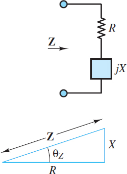
Figure 4 Impedance triangle
Basic trigonometry yields:
\[R=\left| \text{ }\!\!Z\!\!\text{ } \right|\cos \theta \begin{matrix}{} & (15) \\\end{matrix}\]
\[X=\left| \text{ }\!\!Z\!\!\text{ } \right|\sin \theta \begin{matrix}{} & (16) \\\end{matrix}\]
where R is the resistance and X is the reactance. Notice that both R and Pavg are proportional to cos (𝜃Z), which suggests that a triangle similar to (i.e., the same shape as) the impedance triangle could be constructed with Pavg as one leg of a right triangle. In fact, such a triangle is known as a power triangle. The similarity of these two types of triangles is a powerful concept for problem solving.
Power Factor
The phase angle 𝜃Z of the load impedance plays a very important role in AC power circuits. From equation 12, the average power dissipated by an AC load is proportional to cos (𝜃Z). For this reason, cos (𝜃Z) is known as the power factor (pf). For purely resistive loads:
\[\begin{matrix}{{\theta }_{Z}}=0 & \to & pf=1 & \begin{matrix}\text{Resistive Load} & (17) \\\end{matrix} \\\end{matrix}\]
For purely inductive or capacitive loads:
\[\begin{matrix}{{\theta }_{Z}}=+\pi /2 & \to & pf=0 & \begin{matrix}Inductive\text{ }Load & (18) \\\end{matrix} \\\end{matrix}\]\[\begin{matrix}{{\theta }_{Z}}=-\pi /2 & \to & pf=0 & \begin{matrix}Capacitive\text{ }Load & (19) \\\end{matrix} \\\end{matrix}\]
For loads with non-zero resistive (real) and reactive (imaginary) parts:
\[\begin{matrix}0<\left| {{\theta }_{Z}} \right|<\pi /2 & \to & \begin{matrix}0<pf<1 & \begin{matrix}Complex\text{ }Load & (20) \\\end{matrix} \\\end{matrix} \\\end{matrix}\]
Using the definition pf = cos(𝜃Z) the average power can be expressed as:
\[{{P}_{avg}}=\overset{\tilde{\ }}{\mathop{V}}\,\overset{\tilde{\ }}{\mathop{I}}\,pf\begin{matrix}{} & {} & (21) \\\end{matrix}\]
Thus, average power dissipated by a resistor is:
\[{{({{P}_{avg}})}_{R}}=\overset{\tilde{\ }}{\mathop{{{V}_{R}}}}\,\overset{\tilde{\ }}{\mathop{{{I}_{R}}}}\,p{{f}_{R}}=\overset{\tilde{\ }}{\mathop{{{V}_{R}}}}\,\overset{\tilde{\ }}{\mathop{{{I}_{R}}}}\,\begin{matrix}{} & (22) \\\end{matrix}\]
Because pfR = 1. By contrast, the average power dissipated by a capacitor or inductor is:
\[{{({{P}_{avg}})}_{X}}=\overset{\tilde{\ }}{\mathop{{{V}_{X}}}}\,\overset{\tilde{\ }}{\mathop{{{I}_{X}}}}\,p{{f}_{X}}=0\begin{matrix}{} & (23) \\\end{matrix}\]
Because pfX = 0, where the subscript X indicates a reactive element (i.e., either a capacitor or inductor). It is important to note that although capacitors and inductors are lossless (i.e., they store and release energy but do not dissipate energy), they do influence power dissipation in a circuit by affecting the voltage across and the current through resistors in the circuit.
When θz is positive, the load is inductive and the power factor is said to be lagging; when θz is negative, the load is capacitive and the power factor is said to be leading.
It is important to keep in mind that pf = cos(θZ) = cos(−θZ) because the cosine is an even function. Thus, while it may be important to know whether a load is inductive or capacitive, the value of the power factor only indicates the extent to which a load is inductive or capacitive.
To know whether a load is inductive or capacitive, one must know whether the power factor is leading or lagging.
Instantaneous and Average Power Key Takeaways
Understanding power calculations in AC circuits is essential for designing and optimizing electrical systems. Concepts such as instantaneous and average power, root mean square (rms) values, impedance, and power triangles directly impact how energy is managed in various applications. For instance, calculating average power helps in determining energy consumption and system efficiency, while the power factor influences the overall performance of electrical devices. By analyzing phase relationships, impedance, and voltage-current interactions, engineers can better design circuits that minimize energy loss and maximize efficiency, crucial for everything from residential power systems to industrial machinery.