The article discusses the frequency response of a second-order RLC band pass filter, explaining how it allows signals within a specific frequency range to pass while attenuating frequencies outside that range. It also explores key concepts such as resonance, bandwidth, quality factor, and damping ratio, and how they influence the filter’s performance.
Using the same principles and procedures in the case of low and high pass filters, it is possible to derive a band pass filter frequency response for particular types of circuits. Such a filter passes the input to the output at frequencies within a certain range. The analysis of a simple second-order (i.e., two energy storage elements) bandpass filter is similar to that of low and high pass filters. Consider the circuit shown in Figure 1 and the designated frequency response function:
\[H (j\omega )=\frac{{{V}_{0}}}{{{V}_{i}}}(j\omega )\]
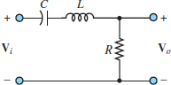
Figure 1 RLC bandpass filter.
Apply voltage division to find:
\[\begin{matrix}{{V}_{0}}(j\omega )={{V}_{i}}(j\omega )\frac{R}{R+1/j\omega C+j\omega L} & {} & {} \\{} & {} & (1) \\={{V}_{i}}(j\omega )\frac{j\omega CR}{1+j\omega CR+{{(j\omega )}^{2}}LC} & {} & {} \\\end{matrix}\]
Thus, the frequency response function is:
\[\frac{{{V}_{0}}}{{{V}_{i}}}(j\omega )=\frac{j\omega CR}{1+j\omega CR+{{(j\omega )}^{2}}LC}\begin{matrix}{} & (2) \\\end{matrix}\]
Equation 2 be factored into the form
\[\frac{{{V}_{0}}}{{{V}_{i}}}(j\omega )=\frac{jA\omega }{(j\omega /{{\omega }_{1}}+1)+(j\omega /{{\omega }_{2}}+1)}\begin{matrix}{} & (3) \\\end{matrix}\]
Where ω1 and ω2 are the two frequencies that determine the passband (or bandwidth) of the filter—that is, the frequency range over which the filter “passes” the input signal—and A is a constant that results from the factoring.
An immediate observation we can make is that if the signal frequency ω is zero, the response of the filter is equal to zero since at ω = 0 the impedance of the capacitor 1/jωC becomes infinite. Thus, the capacitor acts as an open-circuit, and the output voltage equals zero.
Further, we note that the filter output in response to an input signal at sinusoidal frequency approaching infinity is again equal to zero. This result can be verified by considering that as ω approaches infinity, the impedance of the inductor becomes infinite, that is, an open-circuit. Thus, the filter cannot pass signals at very high frequencies.
In an intermediate band of frequencies, the bandpass filter circuit will provide a variable attenuation of the input signal, dependent on the frequency of the excitation. This may be verified by taking a closer look at equation 1:
\[\begin{matrix}H (j\omega )=\frac{{{V}_{0}}}{{{V}_{i}}}(j\omega )=\frac{jA\omega }{(j\omega /{{\omega }_{1}}+1)+(j\omega /{{\omega }_{2}}+1)} & {} & {} \\=\frac{A\omega {{e}^{j\pi /2}}}{\sqrt{1+{{(\omega /{{\omega }_{1}})}^{2}}}\sqrt{1+{{(\omega /{{\omega }_{2}})}^{2}}}{{e}^{j\arctan (\omega /{{\omega }_{1}})}}{{e}^{j\arctan (\omega /{{\omega }_{2}})}}} & {} & \left( 4 \right) \\=\frac{A\omega }{\sqrt{\left[ 1+{{(\omega /{{\omega }_{1}})}^{2}} \right]\left[ 1+{{(\omega /{{\omega }_{2}})}^{2}} \right]}}{{e}^{j\left[ \pi /2-\arctan (\omega /{{\omega }_{1}})-\arctan (\omega /{{\omega }_{2}}) \right]}} & {} & {} \\\end{matrix}\]
Equation 2 is of the form H (jω) =|H|ej∠H, with
\[\begin{matrix} \begin{align} & \left| H (j\omega ) \right|=\frac{A\omega }{\sqrt{\left[ 1+{{(\omega /{{\omega }_{1}})}^{2}} \right]\left[ 1+{{(\omega /{{\omega }_{2}})}^{2}} \right]}} \\ & \angle H (j\omega )=\frac{\pi }{2}-\arctan \frac{\omega }{{{\omega }_{1}}}-\arctan \frac{\omega }{{{\omega }_{2}}} \\\end{align} & {} & (5) \\\end{matrix}\]
The magnitude and phase plots for the frequency response of the bandpass filter of Figure 1 are shown in Figure 2. These plots have been normalized to have the filter passband centered at the frequency ω = 1 rad/s.
The frequency response plots of Figure 2 suggest that, in some sense, the band pass filter acts as a combination of a high-pass and a low-pass filter. As illustrated in the previous cases, it should be evident that one can adjust the filter response as desired simply by selecting appropriate values for L, C, and R.
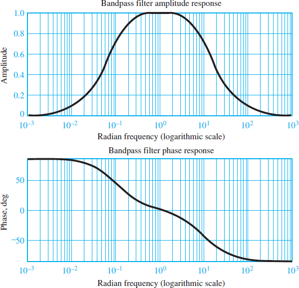
Figure 2 Frequency response of RLC band pass filter
Resonance and Bandwidth
The response of second-order filters can be explained more generally by rewriting the frequency response function of the second-order bandpass filter of Figure 1 in the following forms:
\[\begin{matrix}\frac{{{V}_{0}}}{{{V}_{_{i}}}}(j\omega )=\frac{j\omega CR}{LC{{(j\omega )}^{2}}+j\omega CR+1} & {} & {} \\=\frac{(2\zeta /{{\omega }_{n}})j\omega }{{{(j\omega /{{\omega }_{n}})}^{2}}+(2\zeta /{{\omega }_{n}})j\omega +1} & {} & (6) \\=\frac{(1/Q{{\omega }_{n}})j\omega }{{{(j\omega /{{\omega }_{n}})}^{2}}+(1/Q{{\omega }_{n}})j\omega +1} & {} & {} \\\end{matrix}\]
with the following definitions:
\[\begin{matrix}{{\omega }_{n}}=\sqrt{\frac{1}{LC}}=natural\begin{matrix}or\begin{matrix}resonant\begin{matrix}frequency \\\end{matrix} \\\end{matrix} \\\end{matrix} & {} & {} \\Q=\frac{1}{2\zeta }=\frac{1}{{{\omega }_{n}}CR}={{\omega }_{n}}\frac{L}{R}=\frac{1}{R}\sqrt{\frac{L}{C}}=quality\text{ }factor & {} & (7) \\\zeta =\frac{1}{2Q}=\frac{R}{2}\sqrt{\frac{C}{L}}=damping\text{ }ratio & {} & {} \\\end{matrix}\]
Figure 3 depicts the normalized frequency response (magnitude and phase) of the second-order band pass filter for ωn = 1 and various values of Q (and ζ). The peak displayed in the frequency response around the frequency ωn is called a resonant peak, and ωn is the resonant frequency.
Note that as the quality factor Q increases, the sharpness of the resonance increases and the filter becomes increasingly selective (i.e., it has the ability to filter out most frequency components of the input signals except for a narrow band around the resonant frequency).
One measure of the selectivity of a bandpass filter is its bandwidth. The concept of bandwidth can be easily visualized in the plot of Figure 3(a) by drawing a horizontal line across the plot (we have chosen to draw it at the amplitude ratio value of 0.707 for reasons that will be explained shortly). The frequency range between (magnitude) frequency response points intersecting this horizontal line is defined as the half-power bandwidth of the filter.
The name half-power stems from the fact that when the amplitude response is equal to 0.707 (or ${}^{1}/{}_{\sqrt{2}}$ ), the voltage (or current) at the output of the filter has decreased by the same factor, relative to the maximum value (at the resonant frequency). Since power in an electric signal is proportional to the square of the voltage or current, a drop by a factor ${}^{1}/{}_{\sqrt{2}}$ in the output voltage or current corresponds to the power being reduced by a factor of ½.
Thus, we term the frequencies at which the intersection of the 0.707 line with the frequency response occurs the half-power frequencies. Another useful definition of bandwidth B is as follows. Note that a high-Q filter has a narrow bandwidth and a low- Q filter has a wide band with.
\[B=\frac{{{\omega }_{n}}}{Q}\begin{matrix}{} & Ban{{d}_{{}}}width & \begin{matrix}{} & (8) \\\end{matrix} \\\end{matrix}\]
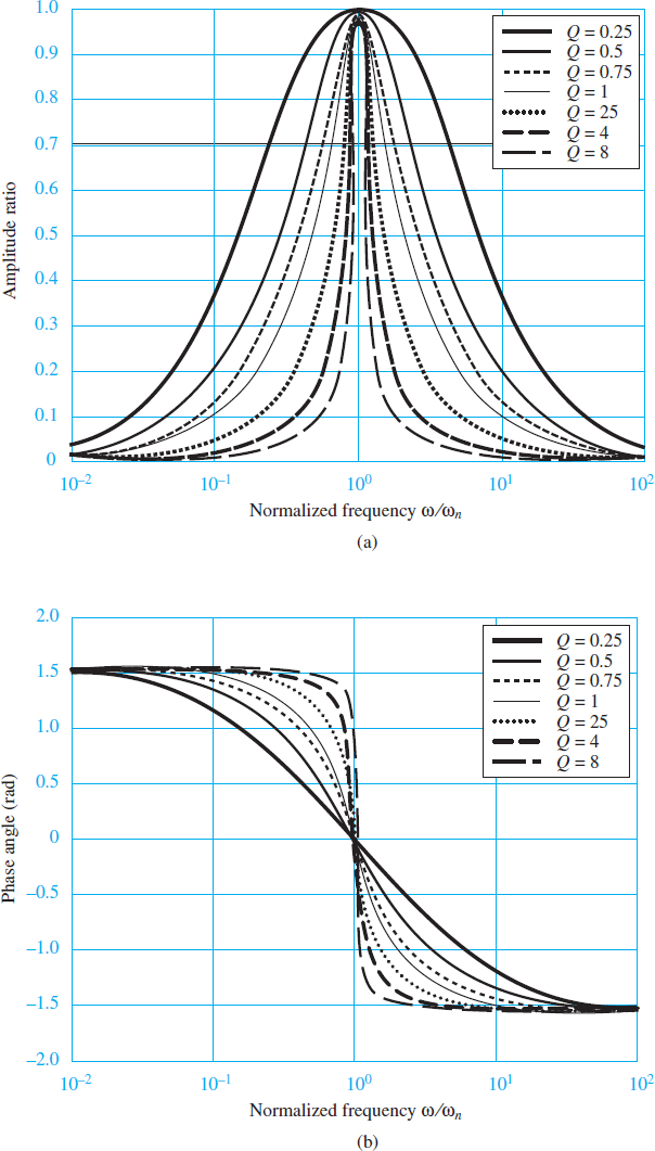
Figure 3(a) Normalized magnitude response of second-order bandpass filter; (b) normalized phase response of second-order bandpass filter
Band Pass Filter Frequency Response Key Takeaways
Understanding the frequency response of a second-order RLC band pass filter is crucial due to its wide range of practical applications in signal processing and communication systems. By allowing only a specific range of frequencies to pass while attenuating all others, such filters are essential in tasks like noise reduction, signal selection, and frequency tuning. Key parameters like resonance, bandwidth, quality factor (Q), and damping ratio (ζ) enable engineers to tailor a filter’s performance to specific application needs—whether it’s isolating a communication channel, designing audio equipment, or processing biomedical signals. The ability to control these characteristics through component values (R, L, C) makes RLC bandpass filters powerful and adaptable tools in modern electronic circuit design.