Transistor Amplifier Coupling Methods: Transformer, RC, Direct, and Push-Pull Coupling
Learn about the four main transistor amplifier coupling methods: transformer, RC, direct, and push-pull coupling, including their operating principles, impedance matching, and applications.
Transistor stages can be connected in series to produce the desired amplification. Connecting these stages in series is called cascading. The key challenge of cascading is matching the high impedance output of one transistor to the low input impedance of the next transistor without severe loss in gain.
Transistor stages can be connected using one of the four primary methods:
- Transformer coupling.
- RC coupling.
- Direct coupling.
- Push-pull coupling.
Transformer Coupling
The circuit in Figure 1 shows two stages of transistor amplifier coupled with a transformer. Transistor Q1 has an output impedance of 20 kΩ, and Q2 has an input impedance of 1 kΩ. A severe mismatch and loss of gain results when they are directly connected. The purpose of capacitor C in the transformer coupling circuit of Figure 1 is to block the DC bias voltage of the transistor from ground. Notice that if C is left out, the transistor base will be grounded directly through the transformer secondary.
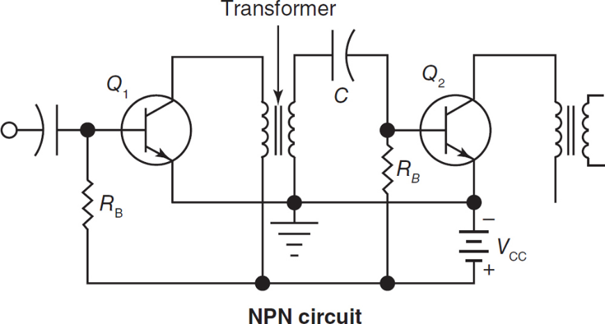
Figure 1. Transformer coupled amplifier circuit.
A transformer can match these impedances. In this case, a step-down transformer is required. A low secondary voltage means a higher secondary current. This condition is acceptable for transistors because they are current operated. Many special sub-ouncer and sub-sub-ouncer transformers have been developed for this purpose, Figure 2.
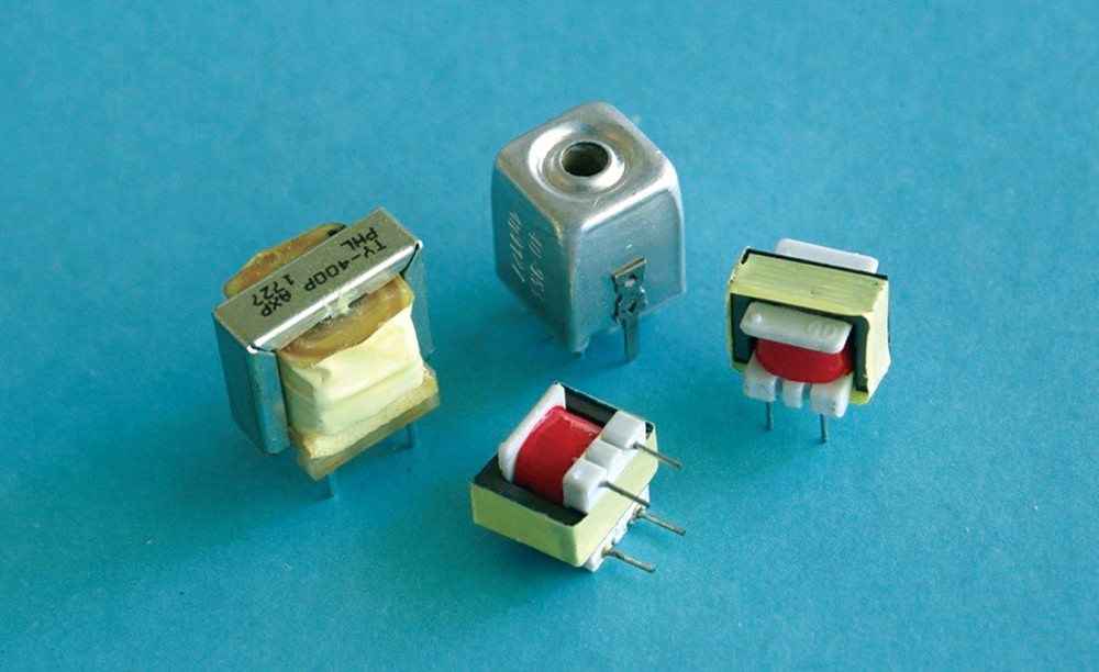
Figure 2. Typical audio transformers, also known as sub-ouncer transformers.
The major drawback of transformer coupling, besides the cost, is the poor frequency response of transformers. They tend to saturate at high audio frequencies. At radio frequencies, inductance and winding capacitance present problems.
A type of transformer coupling that avoids this problem uses a tapped transformer. These taps can be at medium, low, and high impedance points. Good impedance matching can be attained with taps, as well as good coupling and gain. Study the circuit in Figure 3. For radio frequency amplifier circuits, both the transformer primary and secondary windings can be tuned by variable capacitors for frequency choice.
There is one other key point about the transformer. The primary impedance of the transformer acts as a collector load for the transistor. This impedance only appears under signal conditions. The load is XL of primary. From the DC point of view, the only load is the ohmic resistance of the wire used to wind the transformer primary. This information will be helpful when designing a power amplifier.
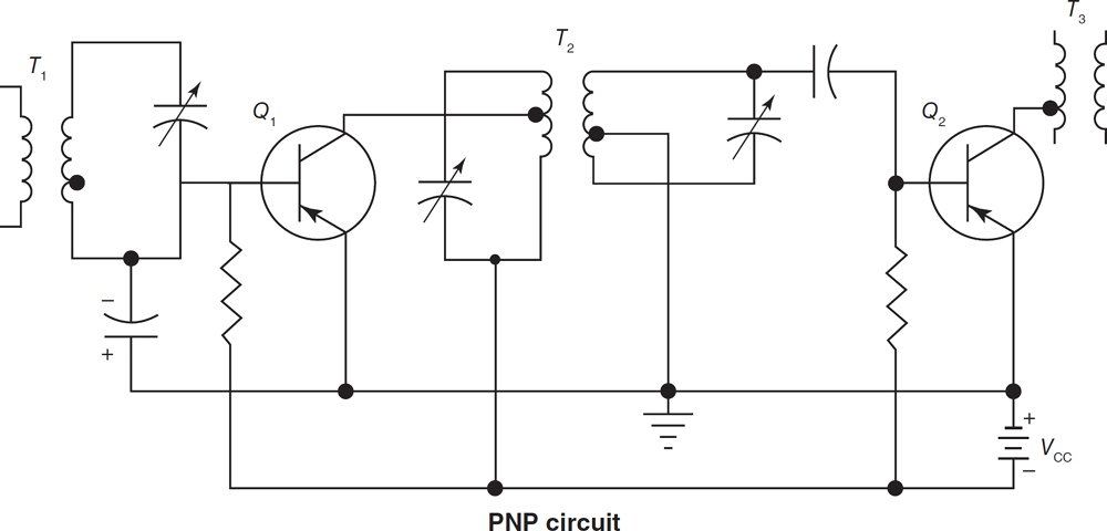
Figure 3. The taps on the transformer primary and secondary windings provide an ideal matching point. The transformer can be designed for good overall gain.
RC Coupling
A simple and less costly method of coupling transistor amplifier stages is to use resistor-capacitor (RC) coupling. See Figure 4.
In Figure 4A, capacitor C charges to 10 volts. Only during the charging of C will a current cause a voltage to appear across R. After C is charged, VC will equal 10 volts, and VR will equal zero.
If the source voltage is changed to 12 volts, VC will also increase to 12 volts, Figure 4B. The charging current will produce a brief two-volt pulse across R in the polarity shown.
If the source voltage is changed to eight volts, C will discharge to eight volts, Figure 4C. The discharge current will produce a brief voltage pulse across R in the polarity shown.
In Figure 4D, both DC and AC voltages are connected to the RC circuit. The AC signal causes the total voltage to vary between 8 and 12 volts. Therefore, C charges and discharges at the AC generator frequency.
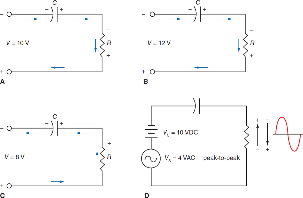
Figure 4. Coupling transistor amplifier using RC coupling.
The voltage across R rises and falls at the same frequency as the generator voltage. Refer to Figure 5. The input signal varies around a DC level of 10 volts. But the output signal varies around the zero-volt level. The DC component has been removed. A capacitor blocks DC. A capacitor used to block DC is called a blocking capacitor.
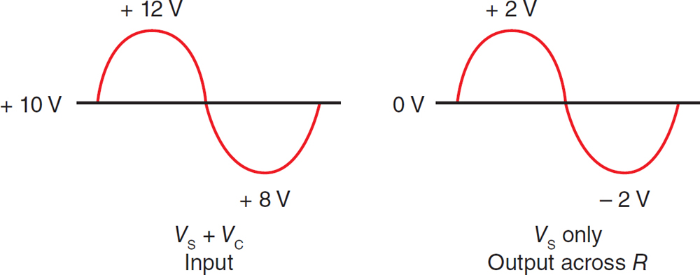
Figure 5. The capacitor blocks the DC voltage, but permits the AC signal to pass.
From a mathematical viewpoint, C and R in series form an AC voltage divider, Figure 6. Voltage division depends on the reactance of XC at the frequency of the signal. Voltage output across R is a key consideration when the greatest amount of AC voltage must appear across R. With a 1,000 Hz frequency signal and a C value of 0.01 µF:
$$X_C=\frac{1}{2\pi fC}=\frac{1}{6.28\times10^3\,\text{Hz}\times1\times10^{-8}\,\text{F}}\cong0.16\times10^5\,\Omega=16,000\,\Omega$$
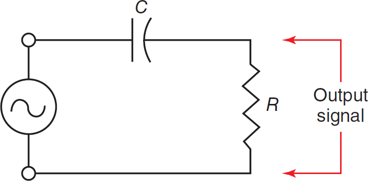
Figure 6. R and C form a voltage divider for the AC signal.
If the value of R is ten or more times greater than XC, then most of the voltage will appear across R. Assuming R equals 160 kΩ, then:
$$V_R=\left(\frac{R}{R+X_C}\right)\times V_{in}=\left(\frac{1.6\times10^5\,\Omega}{(1.6\times10^5\,\Omega)+(1.6\times10^4\,\Omega)}\right)\times V_{in}=\left(\frac{1.6\times10^5\,\Omega}{1.6\times10^4\,\Omega}\right)\times V_{in}=0.91\times10\,V=9.1\,V$$
It seems that almost all of the voltage appears across R. Less than a volt has been lost as signal output. If R were made larger, then even more of the total output would be developed across R.
Refer to the two-stage amplifier using transistors in Figure 7. Consider the signal voltage at the collector of Q1. There is more than one path for the voltage, and it will always take the easiest path. It can go through RC or through the coupling network that is in parallel. If the network impedance is higher than RC, signal currents will go through RC instead of to the next stage. Therefore, the coupling capacitors used in transistor circuits must have values in the range of 8 to 10 µF.
To prove the point, assume Q2 input impedance is 500 W. XC would need to be 50 Ω or less. At 1,000 Hz frequency:
$$C=\frac{1}{2\pi fX_C}=\frac{1}{6.28\times10^3\,\text{Hz}\times50\,\Omega}\cong3.2\,\mu\text{F}$$
At lower amplified frequencies, XC would be higher. A capacitor of 8 to 10 mF would be required to prevent loss of amplifier gain.
Note also in Figure 7 that RF and RB are in parallel with the emitter-base circuit. These resistor values must be high enough so that the signal will not be bypassed around the emitter junction.
The values of RB and RF are based on the required bias and stability of the circuit. Current drain from the source is also considered.
Transistor circuit design can become quite complex and is often a matter of give and take. Compare the output and input impedances of the transistors in the CE configuration. The input can be in the 500 to 1.5 kΩ range. The output impedance is in the 30 kΩ to 50 kΩ range. This is a severe mismatch. With the RC coupling, the loss of power gain caused by the mismatch must be accepted. When cost is a factor, it may be cheaper to add another transistor stage. This addition will offset the loss due to mismatch and is less costly than purchasing a transformer for interstage matching.
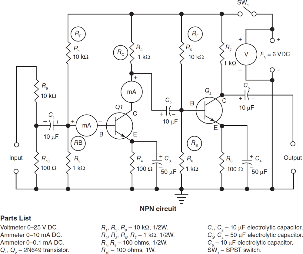
Figure 7. Schematic and parts list for RC coupling.
Direct Coupling
In many circuits, very low frequency signals must be amplified or, perhaps, the DC value of a signal must be retained. Amplifier circuits using RC or transformer coupling block out the DC component. Direct coupling solves this problem, Figure 8.
In this circuit, the collector of Q1 is joined directly to the base of Q2. Collector load resistor RC also acts as a bias resistor for Q2.
However, any change of bias current is amplified by the directly coupled circuit. This creates sensitivity to any temperature changes. This can be overcome with stabilizing circuits. Another drawback of direct coupling is that each stage needs a different bias voltage for proper operation.
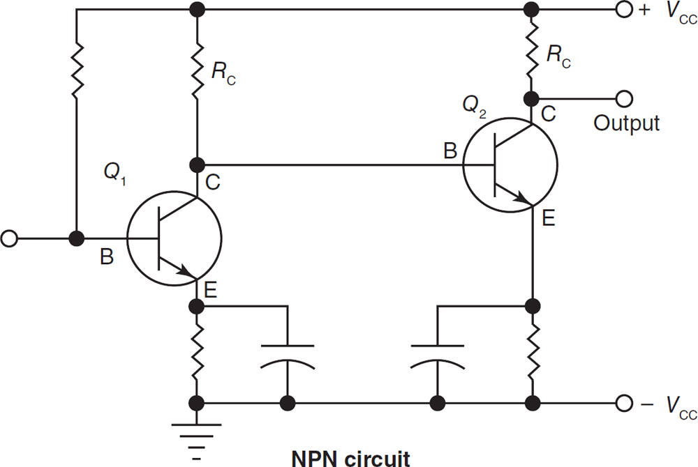
Figure 8. Directly coupled amplifier.
Push-Pull Coupling
Two transistors joined in parallel in a push-pull power amplifier circuit will achieve peak power output and efficiency from a power amplifier, Figure 9.
This basic circuit works at zero bias when no signal is applied. No voltage is applied across the EB junction, so the current IB is zero. When point A of the input transformer becomes negative (result of a signal), then B of Q1 is more negative than E. This is a forward bias and Q1 conducts. At the same time, the base of Q2 is being driven positive. This action increases the reverse bias on Q2, and Q2 does not conduct.
On the second half of the input signal, the reverse is true. Q2 is driven into conduction when a negative signal is applied to its base. Q1 is cut off as a reverse bias is applied by a positive signal to its base. So, Q1 conducts first, then Q2 conducts.
On one-half cycle, current IC flows in Q1. On the second half cycle, current IC flows in Q2. These transistors are operating Class B. One-half of the time each transistor is resting and cooling. This circuit definitely has increased efficiency. In fact, the maximum possible efficiency approaches 78.5%.
The two half signals, or waves of current, from the transistors are restored to their original input form by transformer action in the output transformer.
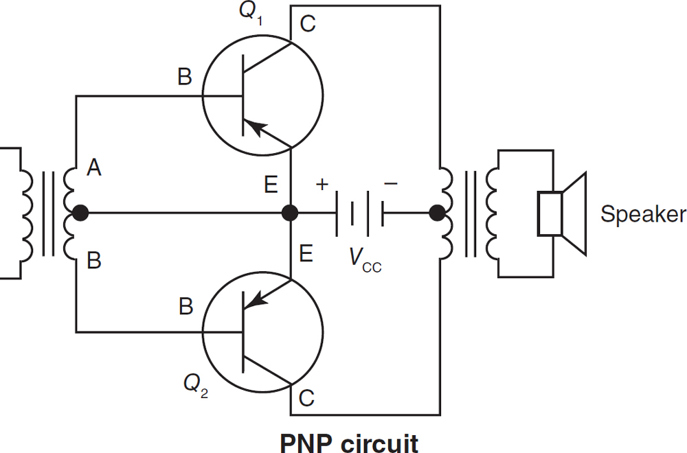
Figure 9. Push-pull amplifier circuit.
In Figure 10, when Q1 conducts, current flows as shown by arrows. It creates a magnetic field of one polarity. This denotes a half-wave form in the secondary of the transformer. When Q2 conducts, the polarity of the primary reverses. It induces the wave of opposite polarity in the secondary. Thus, the complete wave is restored.
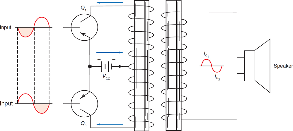
Figure 10. Each half of the signal is joined in the output transformer to restore the original wave.
Impedance Matching
Impedance matching is the practice of matching the output impedance of one device to the input impedance of another electronic device, Figure 11. For the best power transfer, the output impedance of Amplifier A should match the input impedance of Amplifier B. All electronic devices have impedance values. Maximum power transfer occurs when the impedances of the output and input of the two devices match. If the output and input impedances do not match, the most efficient power transfer will not occur and there will be a loss of transfer power.
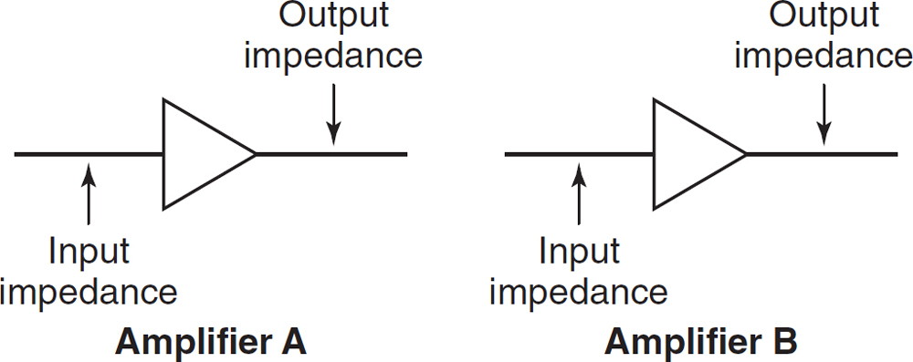
Figure 11. Impedance matching is the practice of matching the output impedance of one electronic device to the input impedance of another electronic device.
Key Takeaways
Transistor amplifier stages can be connected using four primary coupling methods: transformer coupling, RC coupling, direct coupling, and push-pull coupling.
- Transformer coupling provides impedance matching between amplifier stages but has limitations in frequency response and cost.
- RC coupling is simple and economical but introduces gain losses due to impedance mismatch. Direct coupling allows both AC and DC signals to be amplified but is sensitive to temperature and bias variations.
- Push-pull coupling uses two transistors operating alternately in Class B to achieve higher power output and efficiency.
- Impedance matching is an important consideration in multistage amplifiers because it directly affects signal and power transfer between stages.