The article provides an overview of nodal analysis, a method used in electrical circuit analysis that applies Kirchhoff’s current law and source transformation techniques. It also includes a solved example to demonstrate how to apply nodal analysis to calculate currents in a simple circuit.
Nodal analysis is a circuit-analysis format that combines Kirchhoff’s current- law equations with the source transformation. Converting all voltage sources to equivalent constant-current sources allows us to standardize the way we write the Kirchhoff’s current-law equations.
For nodal analysis, we consider source currents to flow into a node. If the arrows in a circuit diagram showing that a source current actually flows out of a particular node, the current is a negative quantity for that node.
Similarly, we consider all resistor currents to flow out of a node. We are thus restating Kirchhoff’s current law in the form:
At any independent node, the algebraic sum of the resistor currents leaving the node equals the algebraic sum of the source currents entering the node.
The Kirchhoff’s current-law equations then have the format
$\begin{matrix} {{I}_{R1}}+{{I}_{R2}}+\cdots ={{I}_{S1}}+{{I}_{S2}}+\cdots & {} & \left( 1 \right) \\\end{matrix}$
The next step is to replace the resistor currents using I = VG.
The voltage across each resistor equals the difference between the voltages, relative to the reference node, of the nodes at each end of the resistor. We always subtract the voltage of the adjacent node from the voltage of the node for which we are writing the equation. For node 1 in
Figure 1, the current through R1 equals V1G1. The voltage across R3 is V1 – V2. Hence the Kirchhoff’s current- law equation for node 1 becomes
${{V}_{1}}{{G}_{1}}+\left( {{V}_{1}}-{{V}_{2}} \right){{G}_{2}}={{I}_{S1}}$
Collecting the voltage terms gives
\[\begin{matrix} \left( {{G}_{1}}+{{G}_{3}} \right){{V}_{1}}-{{G}_{3}}{{V}_{2}}={{I}_{S1}} & {} & \left( 2 \right) \\\end{matrix}\]
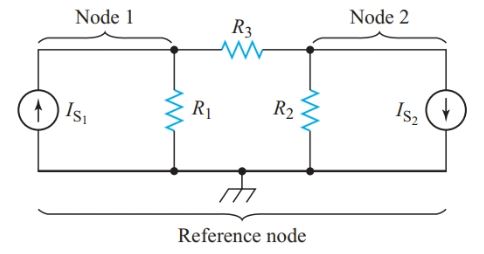
Figure 1 circuit diagram for writing nodal equations
Equation 2 illustrates the standard format for writing a nodal equation. We can use determinants to solve for the voltages.
We can write Equation 2 directly by noting that the positive voltage term on the left-hand side of the equation is the unknown voltage for the node in question multiplied by the sum of the conductance connected to that node. From this positive term, we must subtract a term for the node voltage at every adjacent node connected by a resistor to the node in question. This term is the adjacent node voltage multiplied by the conductance between the two nodes. Using this procedure to write the nodal equation for node 2 gives
\[\left( {{G}_{2}}+{{G}_{3}} \right){{V}_{2}}-{{G}_{3}}{{V}_{1}}=-{{I}_{S2}}\]
Nodal analysis is particularly useful for networks where a common portion of the network is fed from several sources in parallel.
Nodal Analysis Example 1
An automobile generator with an internal resistance of 0.20 V develops an open-circuit voltage of 16.0 V. the storage battery has an internal resistance of 0.10 V and an open-circuit voltage of 12.8 V. Both sources are connected in parallel to a 1.0-V load. Determine the load current.
Solution
Step 1
First, we draw the equivalent circuit with the voltage sources converted to constant-current sources, as shown in Figure 2.
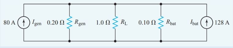
Figure 2 Circuit diagram for Example 1
The short-circuit current for the battery is
\[{{I}_{bat}}=\frac{{{E}_{bat}}}{{{R}_{bat}}}=\frac{12.8V}{0.10\Omega }=128A\]
Similarly, the short-circuit current of the generator is
\[{{I}_{gen}}=\frac{{{E}_{gen}}}{{{R}_{gen}}}=\frac{16V}{0.20\Omega }=80A\]
With a bit of mental arithmetic, we can fill in the required data on the circuit diagram of Figure 2.
Step 2
Next, we find the conductance of each branch:
$\begin{align} & {{G}_{gen}}=\frac{1}{{{R}_{gen}}}=\frac{1}{0.20\Omega }=5S \\ & {{G}_{bat}}=\frac{1}{{{R}_{bat}}}=\frac{1}{0.10\Omega }=10S \\ & and \\ & {{G}_{L}}=\frac{1}{{{R}_{L}}}=1S \\\end{align}$
Step 3
At first glance, Figure 2 appears to show six junction points, but there are only two because the same voltage appears across all parallel branches. For our nodal analysis, we can redraw the circuit in the form shown in Figure 3.
If we label the lower node as the reference node, the upper node is the only independent node. Consequently, we require only one Kirchhoff’s current-law equation for the circuit of Figure 3.
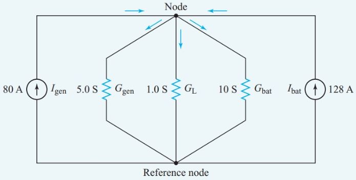
Figure 3 Equivalent circuit for Example 1
At the single independent node, Equation 1 becomes
${{I}_{5}}+{{I}_{1}}+{{I}_{10}}={{I}_{gen}}+{{I}_{bat}}$
Or, we can go directly to the format of Equation 2,
$\begin{align} & \left( {{G}_{5}}+{{G}_{1}}+{{G}_{10}} \right)V={{I}_{gen}}+{{I}_{bat}} \\ & V=\frac{80+128}{5+1+10}=13V \\ & {{I}_{L}}={{G}_{L}}{{V}_{L}}=13V\times 1S=13A \\\end{align}$
The nodal analysis allowed us to solve Example 1 with not much more than mental arithmetic since the circuit has only a single independent node. However, we do need to solve simultaneous equations when the network has more than one independent node.
Nodal Analysis Key Takeaways
Nodal analysis is a powerful and systematic technique essential for analyzing complex electrical circuits, especially when multiple sources are involved. By applying Kirchhoff’s current law and using source transformations, nodal analysis simplifies the process of finding node voltages and branch currents. Its structured approach is particularly advantageous in applications such as power distribution systems, communication networks, and electronic circuit design, where accurate and efficient analysis of interconnected components is crucial. As shown in the example, nodal analysis not only reduces computational effort but also provides clarity in understanding current flow through various branches—making it an indispensable tool in both academic and practical engineering scenarios.