Photovoltaic (PV) System installations constitute a long-term and relatively expensive investment. Therefore, it is essential that an exact design of a certain residential PV installation is carried out.
Figure 1 presents a simple flowchart for the design procedure of residential PV systems. In order to be able to design a PV installation, extensive and precise information of a wide range of parameters are required.
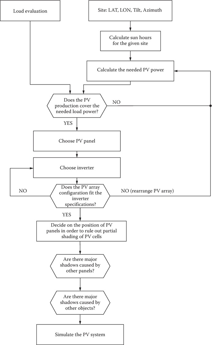
Figure 1 Simple flowchart for a residential PV system design.
Besides all the technical aspects, there are also some financial issues to be considered for such an investment: payback time and internal rate of return.
The financial calculations can be complicated and have many variables included. For small private PV systems on residential houses, the homeowners often look at the investment and the simple payback time in years, which can be calculated as the investment is divided by the yearly savings.
Many homeowners wish to be self-supplied with energy, so the PV system can be dimensioned to cover the annual electricity consumption of the household.
The average energy consumption in a typically Danish four-member family house is approximately 4300 kWh per year.
Depending on the type of feed-in tariff for the produced solar energy, another threshold for the dimension could be the financial optimization of the system.
If the selling price for the produced solar energy is less than the purchase price, many plants are designed to maximize the local consumption of the produced solar power.
As a rule of thumb, a PV plant in Denmark produces 950 kWh per year per installed kWp if all the optimum conditions are met.
In Table 1, this corresponds to an installation at the azimuth of 0 (the azimuth is related to the orientation of the panel and the azimuth angle is 0 if the panels are facing south on the Northern Hemisphere) and a module tilt of 45° (optimum for Denmark).
If the PV Panel is placed with an azimuth of −30° and a module tilt at 0°, the yearly production can roughly be estimated to be (950 kWh × 0.86) ≈ 817 kWh.
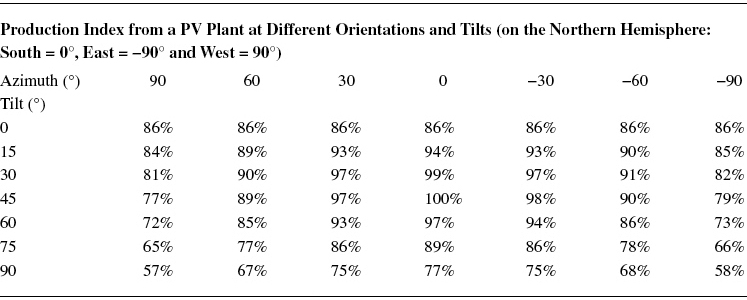
TABLE 1 Deviation from Ideal Production Index in Percent of a PV Panel at Different Orientations and Tilt Angles
Designing the actual PV System begins with choosing the PV module type and the number of modules used in order to achieve the planned amount of kWh, which is followed by the choice of the PV inverter.
On the basis of this information, it will be possible, via a computer and relevant software, to simulate the yield of a certain PV installation with considerable accuracy, depending on the available data.
There are independent software products that can be purchased from several different suppliers, which contain all the required information about PV modules and inverters on the market.
The database within such software is regularly updated with new products. Many inverter manufacturers offer free software for system design. However, these are often restricted to the use of inverters from the inverter supplier, which offers the software tool.
The planning of the PV system in the following text is done with a program supplied for free from the inverter manufacturer SMA and this gives a configuration solution with SMA inverters only.
The case discussed here presents the sizing of a PV system to supply approximately 2500 kWh a year. The system is placed close to the optimum conditions, so the system size can roughly be calculated to 2500 kWh/year divided by the factor 0.95 = 2631 Wp.
The planning is done with a 270 Wp PV module from a Trina-type TSM-270 DC05A.08. The technical data can be seen in Table 2.
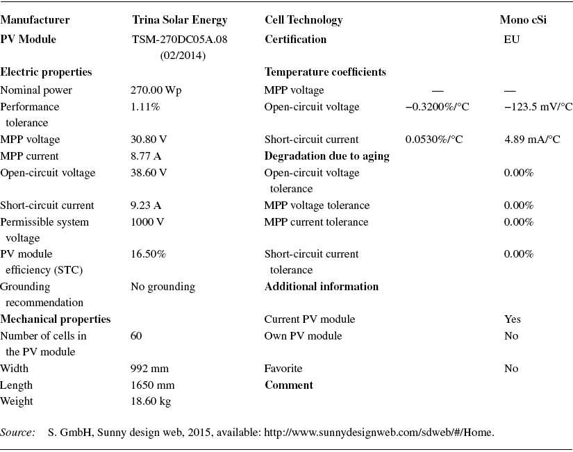
TABLE 2 Datasheet for the Chosen PV Module
Based on the rough size estimation, the number of modules to produce 2500 kWh per year can be calculated: 2631 Wp/270 Wp = 9.74, which if rounded up gives 10 modules.
The first step for the actual design in the program is to create the PV project where all general information about the project is entered:
- Project name
- Customer information
- Project location (for calculating the yield of the system)
- PV plant orientation and tilt
- Installation type (free-standing, roof-integrated, detached on the roof)
After that, the type and numbers of the PV modules are chosen. In this design, there are 10 modules that give the following main plant specifications:
- 10 × 270 Wp = 2700 Wp
- Maximum open-circuit voltage from the system voltage: Voc = 35.8 × 10 = 358 V
- Maximum current in one string: Isc = 7.45 A
When designing PV systems in cold regions, the maximum voltage has to be calculated for −10 °C, whereas the module data are given for +25 °C for most of the cases.
It is important to consider the temperature coefficient of the module, as it can be read from Table 2 to be −0.32%/K. Therefore, the voltage rises in the system due to the low temperature can be calculated as (25+10) ⋅0.32=10.85%, which is automatically given by the software and is an important information based on which the PV inverter is chosen.
As seen in Table 3, the software returns the number of inverters that can be used for the chosen configuration.
For the design presented in this article, the Sunny Boy 2.5-1VL-40 has been chosen. The inverter has a maximum output power of 2.5 kW, while the maximum input voltage is 600 VDC with a maximum current of 10 A.
As seen in the below table, all the design parameters are within the limits of the inverter.
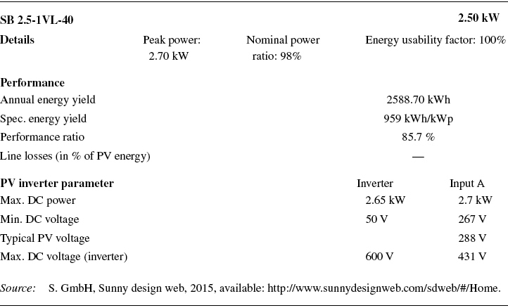
TABLE 3 Specifications Shown for the Chosen PV Inverter
After the selection of the PV inverter, the software returns an overview showing the main technical data for the designed PV system.
The annual yield is calculated to be 2558 kWh with a specific yield per year at 959 kWh/kWp. The inverter is a single-phase inverter, and therefore, the manufacturer highlights that there is 2.5 kVA of unbalanced “load” as seen in Table 4.
Furthermore, the monthly energy productions will also be calculated, and for the presented example, these are given in Figure 2 and Table 5.

TABLE 4 Simple Overview of System Design Showing the Most Important Data for the Designed PV System

Figure 2 Energy production values shown for each month of the year calculated for the 10-panel installation given in Table 4.
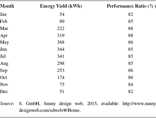
TABLE 5 Calculated Total Energy and Performance Ratio for Each Month Separately for the 10 Panel Installations
The software also allows the user to add and edit several standard parameters such as the cable type and length on both the DC and the AC side, so cable losses can be calculated and taken into account too. The basic formula behind the calculation is as follows:
\[{{P}_{loss}}={{I}^{2}}R\]
Where
Ploss the power loss in the cable (W)
R is the resistance in the cable (Ω)
I is the nominal current in ampere (A)
The resistance R of the cable can be calculated as
\[R=\delta \frac{l}{S}\]
Where
is the resistivity of the material conductor: 0.023 for copper and 0.037 for aluminum (ambient temperature = 25 °C) in
l is the length of the cable in meters (m)
S is the cross section of the cable in (mm2)
A more detailed design software allows the user to build and parametrize custom modules, adjust the PV inverter parameters, calculate and adjust the different losses in the system, and also conduct yield studies, taking into account the module losses placed in shaded positions.
Comments to the Design Differences for TF and Crystalline-Si Systems
A residential PV system consists of several elements that can be categorized into four main topics:
- PV modules—the PV modules on the roof that generate electricity
- PV Inverter—the unit that converts the DC power from the modules to AC power usable in the house
- Balance of system (BOS) components—cable, mounting structure, fuses, etc.
- Labor cost—the cost of installing the system (electrician/carpenter)
Thin Film PV system design is basically similar to c-Si system design methodology; however, due to the lower efficiency and higher output voltage on TF modules, there are some design issues that occur more often when designing smaller systems using this new PV cell technology.
Furthermore, with TF modules, a PV system requires a larger area for the same kWp installation. This also means that there are more BOS components and the labor cost is also higher.
If the same rating of 2.7 kWp is used for the design of a PV system but with TF modules, there will be some differences in the final design.
As an example, one can take the SF 150-S module from Solar Frontier. Its technical specifications are presented in Table 6.
The SF 150-S module has a power output of 150 Wp per module so in this case, 18 modules are needed to reach the target of 2.7 kWp.
Each module has an open-circuit voltage of 108 VDC, and the maximum input voltage of the SMA Sunny Boy 2.5 inverter is 600 VDC, which results in a maximum of 5 series-connected modules to the DC bus of the inverter.
Since the target is 18 modules, one possible configuration is to create 6 parallel strings with 3 modules in series for this inverter. This is not an optimal configuration because more material is needed for the cabling.
Furthermore, a lower input voltage results in the high current, which at the end gives higher losses in the system. This means that another inverter should be used for this particular design case.
Many inverters have a maximum input voltage of 1000 VDC, and by choosing such an inverter, the PR of the designed system could be optimized.
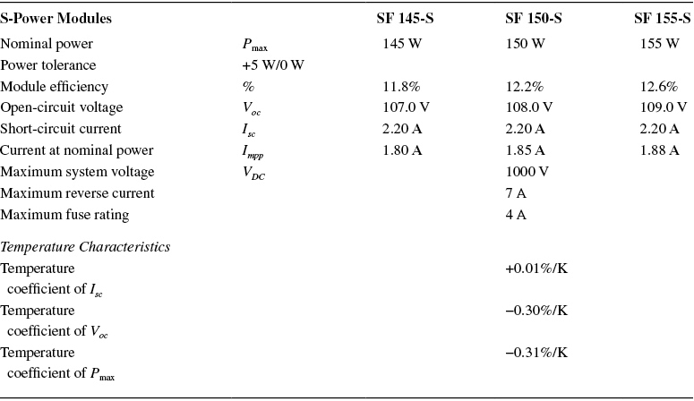
TABLE 6 Solar Frontier, Thin-Film Module Datasheet
PV System Performance Monitoring
When a PV system is installed and commissioned, it is important that the system is properly maintained during its lifetime, which is expected to be above 25 years.
Many PV systems have been sold with the promise that no service or maintenance is needed. This is nearly true. However, faults might appear in the system that will need to be dealt with.
Failure in the different components might happen during the early years of the PV system. Therefore, it is important to know how long the standard warranty period for the different components is.
Warranty of PV Modules
PV modules always come with a limited product warranty; this is typically a 10–15 years’ repair, replacement, or refund remedy. The warranty covers defects in materials and workmanship under normal operating conditions.
There is also a standard in the PV business prescribing that the PV modules are delivered with a limited power warranty. This warranty guarantees that the customer with an output performance of the module in a period up to 30 years depends on the supplier conditions.
The performance warranty typically includes a 10–15 years power guarantee of, for example, 90% of nominal output power and after 25–30 years of operation, 80% power output is guaranteed.
If the power output is below the guaranteed power values, the supplier has to replace such losses in power by either providing the customer additional PV modules to make up for such a loss, by providing monetary compensation equivalent to the cost of the additional PV modules or by repairing or replacing the defective PV modules.
Warranty of PV Inverters
Today, inverters are delivered normally with a minimum of 5 years, warranty. The warranty covers defects in materials and workmanship under normal operating conditions.
Most inverter suppliers offer 5–15 years, extra warranty, which can be purchased before installation or for some suppliers, up to 5 years after the commission of the PV system.
Warranty of BOS Components
BOS components and the installation itself often come with a 10-year warranty. When the PV System is in operation, a minimum of surveillance is needed.
Most new PV inverters today have a built-in Wi-Fi connectivity, so the inverter and the performance of the plant can be monitored through an app or over the Internet.
PV System Price
The price of PV systems has been decreasing since the start of their commercialization back in the 1980s.
The chart in Figure 3 shows both the actual price for c-Si and CdTe for the last 35 years and also the production learning curves when the production is increased.
The actual price follows the learning curve and shows a 22% reduction in price each time the production is doubled.
The pie chart in Figure 4 shows the cost distribution of the major components in the case of a PV system, where the “PV panels” take up 60% and “installation cost” and “installation hardware” take up 15% each, while the “PV inverter” only 10%.
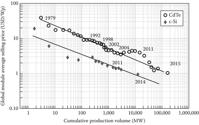
Figure 3 The global PV module price learning curve for c-Si wafer-based and CdTe modules, 1979–2015.
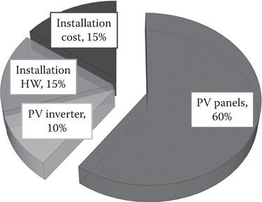
Figure 4 Cost distribution for grid-connected PV systems.
