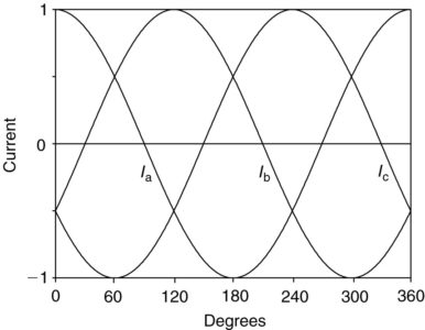
Most of the AC power used today is generated and distributed as three-phase power, which implies three sinusoidal sources, each out of phase with the other. The primary benefit is efficiency: The weight of the conductors and other components in a three-phase system is much lower than that in a single-phase system delivering the same amount of power.
Further, while the power produced by a single-phase system has a pulsating nature a three-phase system can deliver a steady, constant supply of power. For example, later in this article it will be shown that a three-phase generator producing three balanced voltages—that is, voltages of equal amplitude and frequency displaced in phase by 120°—has the property of delivering constant instantaneous power.
The change to three-phase AC power systems from the early DC system proposed by Edison was due to a number of reasons: the efficiency resulting from transforming voltages up and down to minimize transmission losses over long distances, the ability to deliver constant power, a more efficient use of conductors, and the ability to provide starting torque for industrial motors.
Consider a three-phase source connected in a wye (star) configuration, as shown in Figure 1. Each of the three voltages is 120° out of phase with the others, such that:
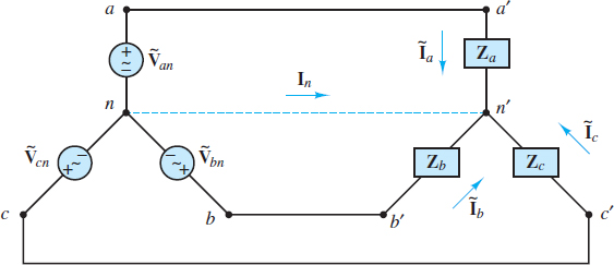
Figure 1 Balanced three-phase AC circuit
\[\begin{matrix}\begin{align}& \overset{\text{ }\!\!\tilde{\ }\!\!\text{ }}{\mathop{{{\text{V}}_{\text{an}}}}}\,=\overset{\tilde{\ }}{\mathop{{{V}_{an}}}}\,\angle {{0}^{^{o}}} \\& \overset{\tilde{\ }}{\mathop{{{\text{V}}_{\text{bn}}}}}\,=\overset{\tilde{\ }}{\mathop{{{V}_{bn}}}}\,\angle -({{120}^{^{o}}}) \\& \overset{\tilde{\ }}{\mathop{{{\text{V}}_{\text{cn}}}}}\,=\overset{\tilde{\ }}{\mathop{{{V}_{cn}}}}\,\angle (-{{240}^{^{o}}})=\overset{\sim }{\mathop{{{V}_{cn}}}}\,\angle {{120}^{o}} \\\end{align} & {} & (1) \\\end{matrix}\]
If the three-phase source is balanced, then:
\[\overset{\text{ }\!\!\tilde{\ }\!\!\text{ }}{\mathop{{{\text{V}}_{\text{an}}}}}\,\text{+}\overset{\text{ }\!\!\tilde{\ }\!\!\text{ }}{\mathop{{{\text{V}}_{\text{bn}}}}}\,\text{+}\overset{\text{ }\!\!\tilde{\ }\!\!\text{ }}{\mathop{{{\text{V}}_{\text{cn}}}}}\,\text{=0}\begin{matrix}{} & Balanced\text{ }phase\text{ }voltages\begin{matrix}{} & {} & (2) \\\end{matrix} \\\end{matrix}\]
The result is the so-called positive abc sequence, as shown in Figure 2. In the wye (star) configuration, the three phase voltages share a common neutral node, denoted by n.
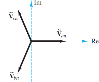
Figure 2 Positive, or abc, sequence for balanced three-phase voltages
It is also possible to define line voltages as the potential differences between lines aa′ and bb′, lines aa′ and cc′, and lines bb′ and cc’. Each line voltage is related to the phase voltages by:
\[\begin{matrix}\overset{\text{ }\!\!\tilde{\ }\!\!\text{ }}{\mathop{{{\text{V}}_{\text{ab}}}}}\,\text{=}\overset{\tilde{\ }}{\mathop{{{\text{V}}_{\text{an}}}}}\,\text{-}\overset{\tilde{\ }}{\mathop{{{\text{V}}_{\text{bn}}}}}\,\text{=}\sqrt{3}\overset{\tilde{\ }}{\mathop{V}}\,\angle {{30}^{o}} & {} & {} \\\overset{\tilde{\ }}{\mathop{{{\text{V}}_{\text{bc}}}}}\,\text{=}\overset{\tilde{\ }}{\mathop{{{\text{V}}_{\text{bn}}}}}\,\text{-}\overset{\tilde{\ }}{\mathop{{{\text{V}}_{\text{cn}}}}}\,=\sqrt{3}\overset{\tilde{\ }}{\mathop{V}}\,\angle (-{{90}^{o}}) & {} & (4) \\\overset{\tilde{\ }}{\mathop{{{\text{V}}_{\text{ca}}}}}\,\text{=}\overset{\tilde{\ }}{\mathop{{{\text{V}}_{\text{cn}}}}}\,\text{-}\overset{\tilde{\ }}{\mathop{{{\text{V}}_{\text{an}}}}}\,=\sqrt{3}\overset{\tilde{\ }}{\mathop{V}}\,\angle {{150}^{o}} & {} & {} \\\end{matrix}\]
It is instructive to note that the circuit of Figure 1 can be redrawn as shown in Figure 3, where it is clear that the three branches are in parallel.
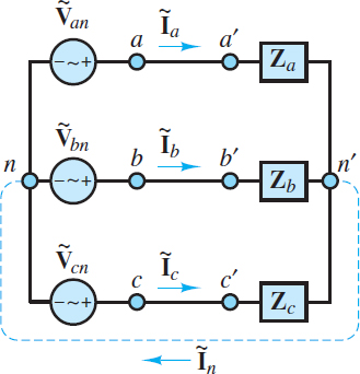
Figure 3 Balanced three-phase AC circuit (redrawn)
When Za = Zb = Zc = Z, the wye (star) load configuration is also balanced. When both the source and load networks are balanced, KCL requires that the current Ĩn in the neutral line n − n′ be identically zero.
\[\overset{\tilde{\ }}{\mathop{{{\text{I}}_{\text{n}}}}}\,\text{=}\overset{\tilde{\ }}{\mathop{{{\text{I}}_{\text{a}}}}}\,\text{+}\overset{\tilde{\ }}{\mathop{{{\text{I}}_{\text{b}}}}}\,\text{+}\overset{\tilde{\ }}{\mathop{{{\text{I}}_{\text{c}}}}}\,\text{=}\frac{\overset{\tilde{\ }}{\mathop{{{\text{V}}_{\text{an}}}}}\,\text{+}\overset{\tilde{\ }}{\mathop{{{\text{V}}_{\text{bn}}}}}\,\text{+}\overset{\tilde{\ }}{\mathop{{{\text{V}}_{\text{cn}}}}}\,}{\text{ }\!\!Z\!\!\text{ }}\text{=0}\begin{matrix}{} & \text{(5)} \\\end{matrix}\]
Another important characteristic of a balanced three-phase power system is illustrated by a simplified version of Figure 3, where the balanced load impedances are replaced by three equal resistors R. Since ?R = 0, the instantaneous power p(t) delivered to each resistor is given by equation [with ?V = ?I and with the freely chosen reference (?V)a = 0)] to be:
\[\begin{matrix}{{p}_{a}}(t)=\frac{\overset{\tilde{\ }}{\mathop{{{V}^{2}}}}\,}{R}(1+\cos 2\omega t) & {} & {} \\{{p}_{b}}(t)=\frac{\overset{\tilde{\ }}{\mathop{{{V}^{2}}}}\,}{R}[(1+\cos (2\omega t-{{120}^{o}})] & {} & (6) \\{{p}_{c}}(t)=\frac{\overset{\tilde{\ }}{\mathop{{{V}^{2}}}}\,}{R}[(1+\cos (2\omega t-{{120}^{o}})] & {} & {} \\\end{matrix}\]
The total instantaneous power p(t) delivered to the total load is the sum:
\[\begin{matrix}p(t)={{p}_{a}}(t)+{{p}_{b}}(t)+{{p}_{c}}(t) & {} & {} \\=\frac{\overset{\tilde{\ }}{\mathop{{{V}^{2}}}}\,}{R}[(3+\cos 2\omega t+\cos (2\omega t-{{120}^{o}})+\cos (2\omega t+{{120}^{o}})] & {} & (7) \\=\frac{\overset{\tilde{\ }}{\mathop{3{{V}^{2}}}}\,}{R}=\text{constant!} & {} & {} \\\end{matrix}\]
It is worthwhile to verify that the sum of the three cosine terms is identically zero. (Hint: Consider the phasor sum of ej(2ωt), ej(2ωt–π/3) and ej(2ωt+π/3).)
Thus, with the simplified balanced resistive load, the total power delivered to the load by the balanced three-phase source is constant. This is an extremely important result, for a very practical reason: Delivering power in a steady fashion (as opposed to the pulsating nature of single-phase power) reduces “wear and tear” on the source and load.
It is also possible to connect three AC sources in a delta (Δ) configuration, as shown in Figure 4 although it is rarely used in practice.
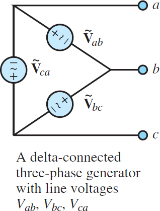
Figure 4 Delta configuration
Balanced Wye (Star) Loads
These results for purely resistive loads can be generalized for any arbitrary balanced complex load. Consider again in Figure 5, where now the balanced load consists of three complex impedances:
\[{{Z }_{a}}={{Z }_{b}}={{Z }_{c}}={{Z }_{y}}=\left| {{Z }_{y}} \right|\angle \theta \begin{matrix}{} & {} & (8) \\\end{matrix}\]
Because of the common neutral line n − n′, each impedance sees the corresponding phase voltage across itself. Therefore, since $\overset{\tilde{\ }}{\mathop{{{V}_{an}}}}\,=\overset{\tilde{\ }}{\mathop{{{V}_{bn}}}}\,=\overset{\tilde{\ }}{\mathop{{{V}_{cn}}}}\,$, it is also true that Ĩa = Ĩb = Ĩc and the phase angles of the currents will differ by ±120°. Consequently, it is possible to compute the power for each phase from the phase voltage and the associated line current. Denote the complex power for each phase by S, where:
\[\begin{matrix}\begin{align}& S=P+jQ \\& \overset{\tilde{\ }}{\mathop{I}}\,\cos \theta +j\overset{\tilde{\ }}{\mathop{V}}\,\overset{\tilde{\ }}{\mathop{I}}\,\sin \theta \\\end{align} & {} & (9) \\\end{matrix}\]
The total real power delivered to the balanced wye (star) load is 3P, and the total reactive power is 3Q. The total complex power ST is
\[\begin{matrix}\begin{align}& {{S}_{T}}={{P}_{T}}+j{{Q}_{T}}=3P+j3Q \\& =\sqrt{{{(3P)}^{2}}+{{(3Q)}^{2}}}\angle \theta \\\end{align} & {} & (10) \\\end{matrix}\]
The apparent power |ST| is:
\[\begin{matrix}\begin{align}& \begin{matrix}\left| {{S}_{T}} \right| & =3\sqrt{{{(\overset{\tilde{\ }}{\mathop{V}}\,\overset{\tilde{\ }}{\mathop{I}}\,)}^{2}}{{\cos }^{2}}\theta +{{(\overset{\tilde{\ }}{\mathop{V}}\,\overset{\tilde{\ }}{\mathop{I}}\,)}^{2}}{{\sin }^{2}}\theta } \\\end{matrix} \\& =3\overset{\tilde{\ }}{\mathop{V}}\,\overset{\tilde{\ }}{\mathop{I}}\, \\\end{align} & {} & (11) \\\end{matrix}\]
Such that:
\[\begin{matrix}\begin{align}& {{P}_{T}}=\left| {{S}_{T}} \right|\cos \theta \\& {{Q}_{T}}=\left| {{S}_{T}} \right|\sin \theta \\\end{align} & {} & (12) \\\end{matrix}\]
Balanced Delta Loads
It is also possible to assemble a balanced load in a delta configuration. A wye (star) generator and a delta load are shown in Figure 5.
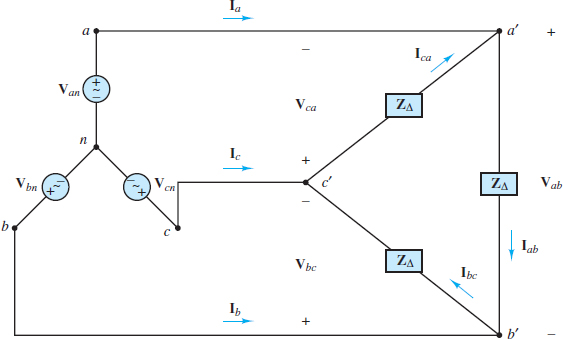
Figure 5 Balanced wye (star) generators with balanced delta load
Note immediately that each impedance ZΔ sees a corresponding line voltage, rather than a phase voltage. For example, the voltage across Zc′a′ is $\overset{\tilde{\ }}{\mathop{{{V}_{ca}}}}\,$. Thus, the three load currents are:
\[\begin{align}& {{\overset{\sim }{\mathop{I }}\,}_{ab}}=\frac{{{\overset{\tilde{\ }}{\mathop{\text{V}}}\,}_{\text{ab}}}}{{{\text{ }\!\!Z\!\!\text{ }}_{\text{ }\!\!\Delta\!\!\text{ }}}}=\frac{\sqrt{3}\overset{\tilde{\ }}{\mathop{V}}\,\angle (\pi /6)}{\left| {{Z }_{\Delta }} \right|\angle \theta } \\& {{\overset{\sim }{\mathop{I }}\,}_{bc}}=\frac{{{\overset{\tilde{\ }}{\mathop{\text{V}}}\,}_{\text{bc}}}}{{{\text{ }\!\!Z\!\!\text{ }}_{\text{ }\!\!\Delta\!\!\text{ }}}}=\frac{\sqrt{3}\overset{\tilde{\ }}{\mathop{V}}\,\angle (-\pi /2)}{\left| {{Z }_{\Delta }} \right|\angle \theta }\begin{matrix}{} & {} & (13) \\\end{matrix} \\& {{\overset{\sim }{\mathop{I }}\,}_{ca}}=\frac{{{\overset{\tilde{\ }}{\mathop{\text{V}}}\,}_{\text{ca}}}}{{{\text{ }\!\!Z\!\!\text{ }}_{\text{ }\!\!\Delta\!\!\text{ }}}}=\frac{\sqrt{3}\overset{\tilde{\ }}{\mathop{V}}\,\angle (5\pi /6)}{\left| {{Z }_{\Delta }} \right|\angle \theta } \\\end{align}\]
The relationship between a delta load and a wye (star) load can be illustrated by determining the delta load ZΔ that would draw the same amount of current as a wye (star) load Zy assuming a given source voltage. Consider the circuits shown in Figures 1 and 5. For instance, the line current drawn in phase a by a wye load is:
\[{{({{\overset{\tilde{\ }}{\mathop{I }}\,}_{a}})}_{y}}=\frac{{{\overset{\tilde{\ }}{\mathop{\text{V}}}\,}_{\text{an}}}}{\text{ }\!\!Z\!\!\text{ }}=\frac{\overset{\tilde{\ }}{\mathop{V}}\,}{\left| {{Z }_{y}} \right|}\angle (-\theta )\begin{matrix}{} & {} & (14) \\\end{matrix}\]
The current drawn by a delta load is:
\[\begin{matrix}\begin{align}& {{\text{(}{{\overset{\text{ }\!\!\tilde{\ }\!\!\text{ }}{\mathop{\text{ }\!\!I\!\!\text{ }}}\,}_{\text{a}}}\text{)}}_{\text{ }\!\!\Delta\!\!\text{ }}}\text{=}{{\overset{\text{ }\!\!\tilde{\ }\!\!\text{ }}{\mathop{\text{ }\!\!I\!\!\text{ }}}\,}_{\text{ab}}}\text{-}{{\overset{\text{ }\!\!\tilde{\ }\!\!\text{ }}{\mathop{\text{ }\!\!I\!\!\text{ }}}\,}_{\text{ca}}} \\& \text{=}\frac{{{\overset{\text{ }\!\!\tilde{\ }\!\!\text{ }}{\mathop{\text{V}}}\,}_{\text{ab}}}}{{{\text{ }\!\!Z\!\!\text{ }}_{\text{ }\!\!\Delta\!\!\text{ }}}}\text{-}\frac{{{\overset{\tilde{\ }}{\mathop{\text{V}}}\,}_{\text{ca}}}}{{{\text{ }\!\!Z\!\!\text{ }}_{\text{ }\!\!\Delta\!\!\text{ }}}} \\& =\frac{\text{1}}{{{\text{ }\!\!Z\!\!\text{ }}_{\text{ }\!\!\Delta\!\!\text{ }}}}\text{(}{{\overset{\tilde{\ }}{\mathop{\text{V}}}\,}_{\text{an}}}\text{-}{{\overset{\tilde{\ }}{\mathop{\text{V}}}\,}_{\text{bn}}}\text{-}{{\overset{\tilde{\ }}{\mathop{\text{V}}}\,}_{\text{cn}}}\text{+}{{\overset{\tilde{\ }}{\mathop{\text{V}}}\,}_{\text{an}}}\text{)} \\& \text{=}\frac{\text{1}}{{{\text{ }\!\!Z\!\!\text{ }}_{\text{ }\!\!\Delta\!\!\text{ }}}}\text{(2}{{\overset{\tilde{\ }}{\mathop{\text{V}}}\,}_{\text{an}}}\text{-}{{\overset{\tilde{\ }}{\mathop{\text{V}}}\,}_{\text{bn}}}\text{-}{{\overset{\tilde{\ }}{\mathop{\text{V}}}\,}_{\text{cn}}}\text{)} \\& =\frac{{{\overset{\tilde{\ }}{\mathop{\text{3V}}}\,}_{\text{an}}}}{{{\text{ }\!\!Z\!\!\text{ }}_{\text{ }\!\!\Delta\!\!\text{ }}}}\text{=}\frac{\text{3}{{\overset{\tilde{\ }}{\mathop{\text{V}}}\,}_{\text{an}}}}{\left| {{\text{ }\!\!Z\!\!\text{ }}_{\text{ }\!\!\Delta\!\!\text{ }}} \right|}\angle \text{(- }\!\!\theta\!\!\text{ )} \\\end{align} & {} & \text{(15)} \\\end{matrix}\]
The two currents (Ĩa)Δ and (Ĩa)y are equal if:
\[{{Z }_{\Delta }}=3{{Z }_{y}}\begin{matrix}{} & {} & (16) \\\end{matrix}\]
This result also implies that a delta load will draw three times as much current and absorb three times as much power as a wye (star) load with the same branch impedance.
