Second Order System Transient Response

In general, a second-order circuit has two irreducible storage elements: two capacitors, two inductors, or one capacitor and one inductor. The latter case is the most important in terms of new fundamentals; however, the important aspects of all second-order system responses are discussed in this section.

Since second-order circuits have two irreducible storage elements, such circuits have two state variables and their behavior is described by a second-order differential equation.

The simplest, yet arguably the most crucial, second-order circuits are those in which the capacitor and inductor are either in parallel or in series, as shown in Figures 1 and 2. The circuits in these figures are drawn to suggest that the capacitor and inductor should be treated as a unified load. The rest of each circuit is either the Thevenin or Norton equivalent of the source network.

The analysis of these circuits is somewhat less complicated than for other second-order circuits, which appealing for anyone learning to analyze such circuits for the first time.

General Characteristics

Before diving into the analysis of particular second-order circuits it is worthwhile to introduce the generalized differential equation for any second-order circuit.

$\begin{matrix}\frac{1}{\omega _{n}^{2}}\frac{{{d}^{2}}x}{d{{t}^{2}}}+\frac{2\zeta }{{{\omega }_{n}}}\frac{dx}{dt}+x={{K}_{s}}f\left( t \right) & {} & \left( 1 \right) \\\end{matrix}$

The constants ω_n and ζ are the natural frequency and the dimensionless damping ratio, respectively. These parameters are characteristics of a second-order circuit and determine its response. Their values will be determined by direct comparison of equation 1 with the differential equation for a specific RLC circuit.

As will be shown, second-order circuits have three distinct possible responses: overdamped, critically damped, and underdamped. The response for any particular second-order circuit is determined entirely by ζ.

In equation 1, f (t ) is a forcing function. K_S is the DC gain of a particular variable x(t). Different variables in the same circuit may have different DC gains. However, all variables share the same natural frequency ω_n, the same dimensionless damping ratio ζ, and therefore also the same type of response. This fact can be important time of server when problem solving.

Parallel LC Circuits

Consider the circuit shown in Figure 1. The two state variables are i_L and v_C, where v_C is the primary state variable because it is shared by all four circuit elements.

In general, at the moment of a transient event the energy of the storage elements may be non-zero; that is, the voltage v_C (0) across the capacitor and the current i_L (0) through the inductor may be non-zero. As always, the two state variables are continuous such that:

$\begin{matrix}{{v}_{C}}\left( {{0}^{+}} \right)={{v}_{C}}\left( {{0}^{-}} \right) & and & {{i}_{L}}\left( {{0}^{+}} \right)={{i}_{L}}\left( {{0}^{-}} \right) \\\end{matrix}$

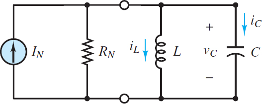
Figure 1 Second-order circuit with the inductor and capacitor in parallel acting as a unified load attached to a Norton equivalent network

Apply KCL to either node to find a first-order differential equation in terms of both state variables.

$\begin{matrix}{{I}_{N}}-\frac{{{v}_{C}}}{{{R}_{N}}}-{{i}_{L}}-{{i}_{C}}=0 & {} & KCL \\\end{matrix}$

The KCL equation can be transformed into a second-order differential equation in i_L by recognizing that:

$\begin{matrix}{{v}_{C}}={{v}_{L}}=L\frac{d{{i}_{L}}}{dt} & and & {{i}_{C}} \\\end{matrix}=C\frac{d{{v}_{C}}}{dt}=LC\frac{{{d}^{2}}{{i}_{L}}}{d{{t}^{2}}}$

Substitute for v_C and i_C in the KCL equation to find:

${{I}_{N}}-\frac{L}{{{R}_{N}}}\frac{d{{i}_{L}}}{dt}-{{i}_{L}}-LC\frac{{{d}^{2}}{{i}_{L}}}{d{{t}^{2}}}=0$

Rearrange the order of terms to yield:

$LC\frac{{{d}^{2}}{{i}_{L}}}{d{{t}^{2}}}+\frac{L}{{{R}_{N}}}\frac{d{{i}_{L}}}{dt}+{{i}_{L}}={{I}_{N}}\begin{matrix}{} & \left( 2 \right) & {} \\\end{matrix}$

Alternatively, one can differentiate both sides of the KCL equation and substitute:

$\begin{matrix}\frac{d{{i}_{L}}}{dt}=\frac{{{v}_{C}}}{L} & and & \frac{d{{i}_{C}}}{dt}=C\frac{{{d}^{2}}{{v}_{C}}}{d{{t}^{2}}} \\\end{matrix}$

The result is:

$\frac{d{{I}_{N}}}{dt}-\frac{1}{{{R}_{N}}}\frac{d{{v}_{C}}}{dt}-\frac{{{v}_{C}}}{L}-C\frac{{{d}^{2}}{{v}_{C}}}{d{{t}^{2}}}=0$

Multiply both sides of the equation by L, and if the source IN is a constant such that its time derivative is zero, the resulting second-order differential equation is:

$\begin{matrix}LC\frac{{{d}^{2}}{{v}_{C}}}{d{{t}^{2}}}+\frac{L}{{{R}_{N}}}\frac{d{{v}_{C}}}{dt}+{{v}_{C}}=0 & {} & \left( 3 \right) \\\end{matrix}$

Equation 3 contains no forcing function (its right side is zero), which indicates that the long-term steady-state solution for v_C will be zero. In other words, the transient solution for v_C is also its complete solution.

To solve equations 2 and 3 it is first necessary to identify the dimension – less damping ratio ζ and the natural frequency ω_n. Notice that the left sides of both equations are identical, as they are for any variable in the circuit. Thus, ω_n and ζ can be found from either differential equation by comparing it to equation 1. The result is:

$\begin{matrix}\frac{1}{\omega _{n}^{2}}=LC & and & \frac{2\zeta }{{{\omega }_{n}}} \\\end{matrix}=\frac{L}{{{R}_{N}}}$

These two equations can be solved to yield:

$\begin{matrix}{{\omega }_{n}}=\frac{1}{\sqrt{LC}} & and & \zeta =\frac{1}{2{{R}_{N}}}\sqrt{\frac{L}{C}} & \left( 4 \right) \\\end{matrix}$

The type of transient response for i_L and v_C depends upon ζ only. When ζ is greater than, equal to, or less than 1, the transient responses (i_L)_TR and (v_C)_TR are overdamped, critically damped, or underdamped, respectively. These three types of responses are described in detail later in this section. The complete solutions are:

${{i}_{L}}\left( t \right)={{\left( {{i}_{L}} \right)}_{TR}}+{{\left( {{i}_{L}} \right)}_{SS}}={{\left( {{i}_{L}} \right)}_{TR}}+{{I}_{N}}$

And

${{v}_{C}}\left( t \right)={{\left( {{v}_{C}} \right)}_{TR}}+{{\left( {{v}_{C}} \right)}_{SS}}={{\left( {{v}_{C}} \right)}_{TR}}+L\frac{d{{I}_{N}}}{dt}$

Note that when I_N is a constant, (v_C )_SS = 0 and v_C (t) = (v_C)_TR(t).

Series LC Circuits

The development of the general solution for series LC circuits follows the same basic steps used above for parallel LC circuits. Consider the circuit in Figure 2 and note the duality between what follows and what was done above for the parallel LC circuit. In fact, the equations that follow can be found simply by starting with the equations developed above and swapping L with C, i_L with v_C , R_N with 1/R_T , and I_N with V_T.

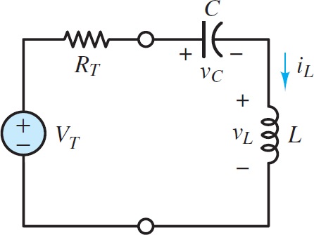
Figure 2 Second-order circuit with the inductor and capacitor in series acting as a unified load attached to a Thevenin equivalent network

Again, the two state variables are i_L and v_C , where i_L is the primary state variable because it is shared by all four circuit elements. Again, at the moment of a transient event the energy of the storage elements may be non-zero; that is, the voltage v_C (0) across the capacitor and the current i_L (0) through the inductor may be non-zero. As always, the two state variables are continuous such that:

$\begin{matrix}{{v}_{C}}\left( {{0}^{+}} \right)={{v}_{C}}\left( {{0}^{-}} \right) & and & {{i}_{L}}\left( {{0}^{+}} \right) \\\end{matrix}={{i}_{L}}\left( {{0}^{-}} \right)$

Apply KVL around the series loop to find a first-order differential equation in terms of both state variables.

$\begin{matrix}{{V}_{T}}-{{i}_{L}}{{R}_{T}}-{{v}_{C}}-{{v}_{L}}=0 & {} & KVL \\\end{matrix}$

The KVL equation can be transformed into a second-order differential equation in v_C by recognizing that:

\[\begin{matrix}{{i}_{L}}={{i}_{C}}=C\frac{d{{v}_{C}}}{dt} & and & {{v}_{L}}=L\frac{d{{i}_{L}}}{dt}=LC\frac{{{d}^{2}}{{v}_{C}}}{d{{t}^{2}}} \\\end{matrix}\]

Substitute for v_L and i_L in the KVL equation to find:

\[{{V}_{T}}-{{R}_{T}}C\frac{d{{v}_{C}}}{dt}-{{v}_{C}}-LC\frac{{{d}^{2}}{{v}_{C}}}{d{{t}^{2}}}=0\]

Rearrange the order of terms to yield:

$\begin{matrix}LC\frac{{{d}^{2}}{{v}_{C}}}{d{{t}^{2}}}+{{R}_{T}}C\frac{d{{v}_{C}}}{dt}+{{v}_{C}}={{V}_{T}} & {} & \left( 5 \right) \\\end{matrix}$

Alternatively, one can differentiate both sides of the KVL equation and substitute:

$\begin{matrix}\frac{d{{v}_{C}}}{dt}=\frac{{{i}_{L}}}{C} & and & \frac{d{{v}_{L}}}{dt}=L\frac{{{d}^{2}}{{i}_{L}}}{d{{t}^{2}}} \\\end{matrix}$

The result is:

$\frac{d{{V}_{T}}}{dt}-{{R}_{_{T}}}\frac{d{{i}_{L}}}{dt}-\frac{{{i}_{L}}}{C}-L\frac{{{d}^{2}}{{i}_{L}}}{d{{t}^{2}}}=0$

Multiply both sides of the equation by C, and if the source V_T is a constant such that its time derivative is zero, the resulting second-order differential equation is:

$\begin{matrix}LC\frac{{{d}^{2}}{{i}_{L}}}{d{{t}^{2}}}+{{R}_{T}}C\frac{d{{i}_{L}}}{dt}+{{i}_{L}}=0 & {} & \left( 6 \right) \\\end{matrix}$

Equation 6 contains no forcing function (its right side is zero), which indicates that the long-term steady-state solution for i_L will be zero. In other words, the transient solution for i_L is also its complete solution.

To solve equations 5 and 6 it is first necessary to identify the dimensionless damping ratio ζ and the natural frequency ω_n. Notice that the left sides of both equations are identical, as they are for any variable in the circuit. Thus, ω_n and ζ can be found from either differential equation by comparing it to equation 1. The result is:

$\frac{1}{\omega _{n}^{2}}=LC\begin{matrix}{} & and & \frac{2\zeta }{{{\omega }_{n}}} \\\end{matrix}={{R}_{T}}C$

These two equations can be solved to yield:

$\begin{matrix}{{\omega }_{n}}=\frac{1}{\sqrt{LC}} & and & \zeta =\frac{{{R}_{T}}}{2} \\\end{matrix}\sqrt{\frac{C}{L}}\begin{matrix}{} & {} & \left( 7 \right) \\\end{matrix}$

The type of transient response for i_L and v_C depends upon ζ only. As al- ways, when ζ is greater than, equal to, or less than 1, the transient responses (i_L)_TR and (v_C )_TR are overdamped, critically damped, or underdamped, respectively. These three types of responses are described in detail later in this section. The complete solutions are:

${{v}_{C}}\left( t \right)={{\left( {{v}_{C}} \right)}_{TR}}+{{\left( {{v}_{C}} \right)}_{SS}}={{\left( {{v}_{C}} \right)}_{TR}}+{{V}_{T}}$

And

${{i}_{L}}\left( t \right)={{\left( {{i}_{L}} \right)}_{TR}}+{{\left( {{i}_{L}} \right)}_{SS}}={{\left( {{i}_{L}} \right)}_{TR}}+C\frac{d{{V}_{T}}}{dt}$

Note that when V_T is a constant, (i_L)_SS = 0 and i_L(t) = (i_L)_TR(t).

Transient Response

The transient response x_TR(t) is found by setting the right side of the governing differential equation equal to zero. That is:

$\begin{matrix}\frac{1}{\omega _{n}^{2}}\frac{{{d}^{2}}{{x}_{TR}}}{d{{t}^{2}}}+\frac{2\zeta }{{{\omega }_{n}}}\frac{d{{x}_{TR}}}{dt}+{{x}_{TR}}=0 & {} & \left( 8 \right) \\\end{matrix}$

Just as in first-order systems, the solution of this equation has an exponential form:

${{x}_{TR}}\left( t \right)=\alpha {{e}^{st}}\begin{matrix}{} & \left( 9 \right) & {} \\\end{matrix}$ Assumed transient response

Substitution into the differential equation yields the characteristic equation:

$\frac{{{s}^{2}}}{\omega _{n}^{2}}+\frac{2\zeta }{{{\omega }_{n}}}+1=0\begin{matrix}   {} & {} & \left( 10 \right)  \\\end{matrix}$

which, in turn, yields two characteristic roots s₁ and s₂. Specific values of s1 and s2 are found from the quadratic formula applied to the characteristic equation:

$\begin{matrix}{{s}_{1,2}}=-\zeta {{\omega }_{n}}\pm \frac{1}{2}\sqrt{{{\left( 2\zeta {{\omega }_{n}} \right)}^{2}}-4\omega _{n}^{2}}=-{{\omega }_{n}}\left( \zeta \pm \sqrt{{{\zeta }^{2}}-1} \right) & {} & \left( 11 \right) \\\end{matrix}$

The roots s₁ and s₂ are associated with the three distinct possible responses: over- damped (ζ > 1), critically damped (ζ = 1), and underdamped (ζ < 1). The details of each of these responses are presented below.

Overdamped Response (ζ > 1)

Two distinct, negative and real roots: (s₁, s₂).The transient response is over-damped when ζ > 1 and the roots are${{s}_{1,2}}={{\omega }_{n}}(-\zeta \pm \sqrt{{{\zeta }^{2}}-1})$. The general form of the solution is:

${{x}_{TR}}\left( t \right)={{\alpha }_{1}}{{e}^{{{s}_{1}}t}}+{{\alpha }_{2}}{{e}^{{{s}_{2}}t}}={{e}^{-\zeta {{\omega }_{n}}t}}\left[ {{\alpha }_{1}}{{e}^{\left( {{\omega }_{n}}\sqrt{{{\zeta }^{2}}-1} \right)t}}+{{\alpha }_{2}}{{e}^{\left( -{{\omega }_{n}}\sqrt{{{\zeta }^{2}}-1} \right)t}} \right]$

$={{\alpha }_{1}}{{e}^{-t/{{\tau }_{1}}}}+{{\alpha }_{2}}{{e}^{-t/{{\tau }_{2}}}}$

$\begin{matrix}{{\tau }_{1}}=\frac{1}{{{\omega }_{n}}\left( \zeta -\sqrt{{{\zeta }^{2}}-1} \right)} & {} & {{\tau }_{2}}=\frac{1}{{{\omega }_{n}}\left( \zeta +\sqrt{{{\zeta }^{2}}-1} \right)} & (12) \\\end{matrix}$

Thus, an overdamped response is the sum of two first-order responses, as shown in Figure 3.

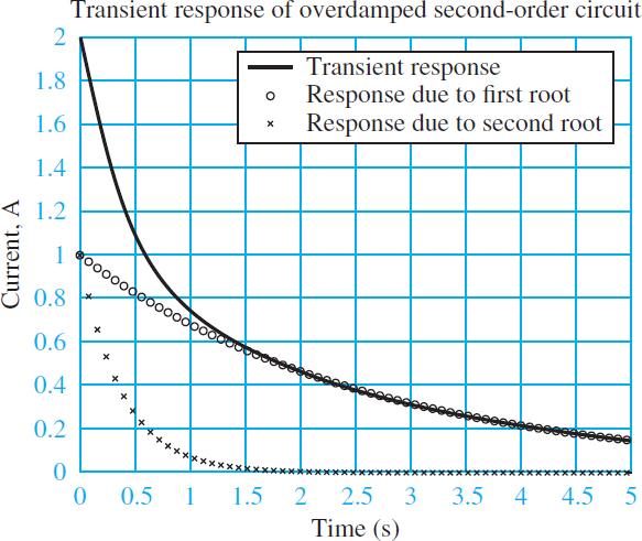
Figure 3 Transient response of underdamped second-order system

Critically Damped Response (ζ = 1)

Two identical, negative, and real roots: (s₁, s₂). The transient response is critically damped when ζ = 1. The general form of the solution is:

${{x}_{TR}}\left( t \right)={{\alpha }_{1}}{{e}^{{{s}_{1}}t}}+{{\alpha }_{2}}t{{e}^{{{s}_{2}}t}}={{e}^{-{{\omega }_{n}}t}}\left( {{\alpha }_{1}}+{{\alpha }_{2}}t \right)={{e}^{-t/\tau }}\left( {{\alpha }_{1}}+{{\alpha }_{2}}t \right)$

$\begin{matrix}\tau =\frac{1}{{{\omega }_{n}}} & {} & \left( 13 \right) \\\end{matrix}$

Note that a critically damped response is the sum of a first-order exponential term plus a similar term multiplied by t. These two components and the complete response are shown in Figure 4.

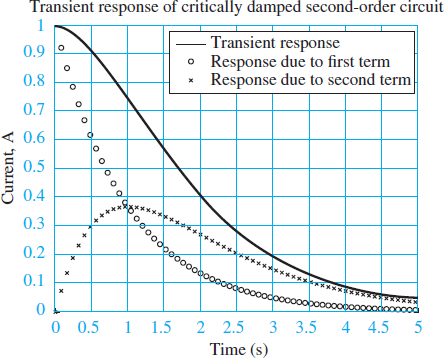
Figure 4 Transient response of a critically damped second-order system

Underdamped Response (ζ < 1)

Two complex conjugate roots: (s₁, s₂). The transient response is underdamped when ζ < 1. The argument of the square root is negative in equation 11, such that ${{s}_{1,2}}={{\omega }_{n}}\left( -\zeta \pm j\sqrt{1-{{\zeta }^{2}}} \right)$ . The following complex exponentials appear in the general form of the response:

$\begin{matrix}{{e}^{^{{{\omega }_{n}}}\left( -\zeta +j\sqrt{1-{{\zeta }^{2}}} \right)t}} & {{e}^{^{{{\omega }_{n}}}\left( -\zeta -j\sqrt{1-{{\zeta }^{2}}} \right)t}} & \left( 14 \right) \\\end{matrix}$

Euler’s formula can be used to express the complex exponentials in terms of sinusoids. The result is:

$\begin{matrix}{{x}_{TR}}\left( t \right)={{e}^{-\zeta {{\omega }_{n}}t}}\left[ {{\alpha }_{1}}\sin \left( {{\omega }_{d}}t \right)+{{\alpha }_{2}}\cos \left( {{\omega }_{d}}t \right) \right] & {} & \left( 15 \right) \\\end{matrix}$

Where ${{\omega }_{d}}={{\omega }_{n}}\sqrt{1-{{\zeta }^{2}}}$ is the damped natural frequency. Note that ω_d is the frequency of oscillation and is related to the period T of oscillation by ω_dT = 2π . Also note that ω_d approaches the natural frequency ω_n as ζ approaches zero. The oscillation is damped by the decaying exponential ${{e}^{-\zeta {{\omega }_{n}}t}}$, which has a time constant$\tau =1/\zeta {{\omega }_{n}}$as shown in Figure 5. As ζ increases toward 1 (more damping), τ decreases and the oscillations decay more quickly. In the limit ζ → 0, the response is a pure sinusoid.

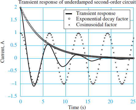
Figure 5 Transient response of an underdamped second-order system for α₁ = α₂ = 1; ζ = 0.2; ω_n = 1

Long-Term Steady-State Response

For switched DC sources, the forcing function F in equation 5.40 is a constant. The result is a constant long-term (t → ∞) steady-state response x_SS.

$\begin{matrix}\frac{1}{\omega _{n}^{2}}\frac{{{d}^{2}}{{x}_{SS}}}{d{{t}^{2}}}+\frac{2\zeta }{{{\omega }_{n}}}\frac{d{{x}_{SS}}}{dt}+{{x}_{SS}}={{K}_{s}}F & {} & \left( 16 \right) \\\end{matrix}$

Since x_SS must also be a constant the solution for x_SS is:

${{x}_{SS}}=x\left( \infty \right)={{K}_{s}}F\begin{matrix}{} & t\to \infty & \left( 17 \right) \\\end{matrix}$

Complete Response

As with first-order systems, the complete response is the sum of the transient and long-term steady-state responses. The complete mathematical solutions for the over- damped, critically damped, and underdamped cases. In each of these cases, the initial conditions on the storage elements must be used to solve for the unknown constants α₁ and α₂. The required procedure uses the two initial conditions to evaluate x(t) and dx/dt at t = 0+. The details of the procedure vary slightly in each of the three cases and are illustrated in the example problems.

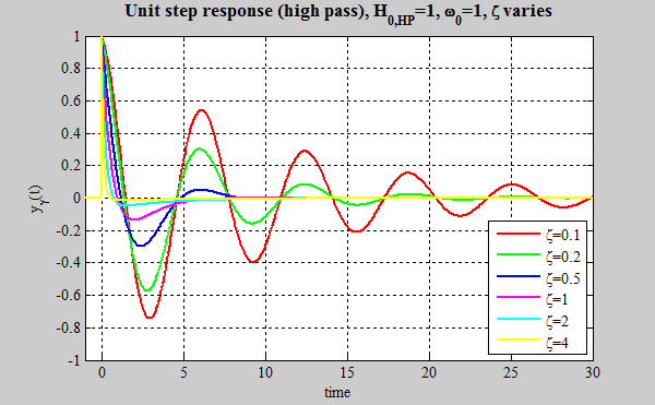
One particularly useful complete solution is the unit-step response brought about by letting K_Sf (t) be a unit step, which equals 0 for t < 0 and 1 for t > 0. To illustrate, assume a dimensionless damping coefficient ζ = 0.1 and an underdamped period of oscillation T = 2π, such that the damped natural frequency is ω_d = 1. The corresponding unit-step response, shown in Figure 6, asymptotically approaches the long-term DC steady-state value of 1 dictated by the unit-step input.

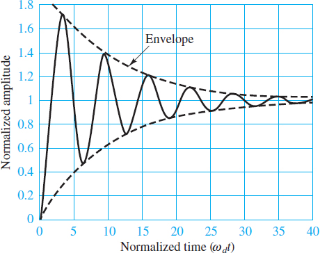
Figure 6 Second order unit step response K_S = 1, ω_d = 1, and ζ = 0.1

Also, as seen in the underdamped transient response, the magnitude of the oscillation’s decays exponentially over time. The time constant for the surrounding envelope.

Note that the rate of decay of the oscillations is governed by ζ. Figure 7 shows that as ζ increases the overshoot of the long-term DC steady-state response decreases until, when ζ = 1 (critically damped), the response no longer oscillates and the overshoot is zero. The response for ζ < 1 (overdamped) has no oscillations and zero overshoot.

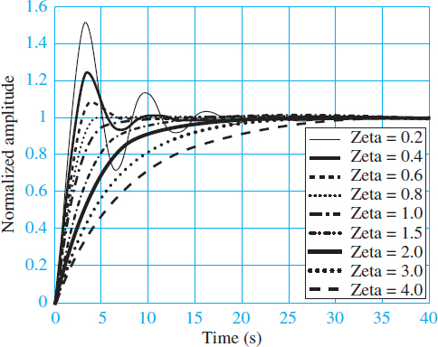
Figure 7 Second-order unit step response K_S = 1, ω_d = 1, and ζ ranging from 0.2 to 4.0