There are many practical applications that involve filters of one kind or another. Modern sunglasses filter out eye-damaging ultraviolet radiation and reduce the intensity of sunlight reaching the eyes. The suspension system of an automobile filters out road noise and reduces the impact of potholes on passengers. An analogous concept applies to electric circuits: it is possible to attenuate (i.e., reduce in amplitude) or al- together eliminate signals of unwanted frequencies, such as those that may be caused by electromagnetic interference (EMI).
Low-Pass Filter Frequency Response
Figure 1 depicts a simple RC filter and denotes its input and output voltages, respectively, by Vi and Vo.
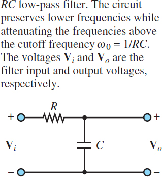
Figure 1 RC Low-pass filter
The frequency response for the filter may be obtained by considering the function
\[H (j\omega )=\frac{{{V}_{0}}}{{{V}_{i}}}\left( j\omega \right)\begin{matrix}{} & (1) \\\end{matrix}\]
and noting that the output voltage may be expressed as a function of the input voltage by means of a voltage divider, as follows
\[{{V}_{0}}(j\omega )={{V}_{i}}(j\omega )\frac{1/j\omega C}{R+1/j\omega C}={{V}_{i}}(j\omega )\frac{1}{1+j\omega RC}\begin{matrix}{} & (2) \\\end{matrix}\]
Thus, the frequency response of the RC filter is
\[\frac{{{V}_{0}}}{{{V}_{i}}}(j\omega )=\frac{1}{1+j\omega CR}\begin{matrix}{} & (3) \\\end{matrix}\]
An immediate observation upon studying this frequency response is that if the signal frequency ω is zero, the value of the frequency response function is 1. That is, the filter is passing all the input. Why? To answer this question, we note that at ω = 0, the impedance of the capacitor, 1/jωC, becomes infinite. Thus, the capacitor acts as an open-circuit, and the output voltage equals the input:
\[{{V}_{0}}(j\omega =0)={{V}_{i}}(j\omega =0)\begin{matrix}{} & (4) \\\end{matrix}\]
Since a signal at sinusoidal frequency equal to zero is a DC signal, this filter circuit does not in any way affect DC voltages and currents. As the signal frequency increases, the magnitude of the frequency response decreases since the denominator increases with ω. More precisely, equations 5 to 8 describe the magnitude and phase of the frequency response of the RC filter:
\[\begin{matrix}H (j\omega )=\frac{{{V}_{0}}}{{{V}_{i}}}(j\omega )=\frac{1}{1+j\omega CR} & {} & {} \\=\frac{1}{\sqrt{1+{{(\omega CR)}^{2}}}}=\frac{{{e}^{j0}}}{{{e}^{-j\arctan (\omega CR/1)}}} & {} & \left( 5 \right) \\=\frac{1}{\sqrt{1+{{(\omega CR)}^{2}}}}{{e}^{-j\arctan (\omega CR)}} & {} & {} \\\end{matrix}\]
OR
\[H (j\omega )=\left| H (j\omega ) \right|{{e}^{j\angle H(j\omega )}}\begin{matrix}{} & (6) \\\end{matrix}\]
WITH
\[\left| H(j\omega ) \right|=\frac{1}{\sqrt{1+{{(\omega CR)}^{2}}}}=\frac{1}{\sqrt{1+{{(\omega /{{\omega }_{0}})}^{2}}}}\begin{matrix}{} & (7) \\\end{matrix}\]
AND
\[\angle H (j\omega )=-\arctan (\omega CR)=-\arctan \frac{\omega }{{{\omega }_{0}}}\begin{matrix}{} & (8) \\\end{matrix}\]
WITH
\[{{\omega }_{0}}=\frac{1}{RC}\begin{matrix}{} & (9) \\\end{matrix}\]
The simplest way to envision the effect of the filter is to think of the phasor voltage scaled by a factor of |H| and shifted by a phase angle ∠H by the filter at each frequency, so that the resultant output is given by the phasor with
\[\begin{matrix}{{V}_{0}}=\left| H \right|.{{V}_{i}} & {} & {} \\{} & {} & (10) \\{{\phi }_{0}}=\angle H +{{\phi }_{i}} & {} & {} \\\end{matrix}\]
and where |H| and ∠H are functions of frequency. The frequency ω0 is called the cutoff frequency of the filter and, as will presently be shown, gives an indication of the filtering characteristics of the circuit.
It is customary to represent H (jω) in two separate plots, representing |H| and ∠H as functions of ω. These are shown in Figure 2 in normalized form, that is, with |H| and ∠H plotted versus ω/ωo, corresponding to a cutoff frequency ω0 = 1 rad/s.
Note that, in the plot, the frequency axis has been scaled logarithmically. This is a common practice in electrical engineering because it enables viewing a very broad range of frequencies on the same plot without excessively compressing the low- frequency end of the plot.
The frequency response plots of Figure 2 are commonly employed to describe the frequency response of a circuit since they can provide a clear idea at a glance of the effect of a filter on an excitation signal. The cutoff frequency ω = 1/RC has a special significance in that it represents approximately the point where the filter begins to filter out the higher-frequency signals. The value of |H (jω)| at the cutoff frequency is ${}^{1}/{}_{\sqrt{2}}=0.707$ . Note how the cutoff frequency depends exclusively on the values of R and C. Therefore, one can adjust the filter response as desired simply by selecting appropriate values for C and R, and therefore one can choose the desired filtering characteristics.
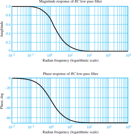
Figure 2 Frequency response of an RC low-pass filter
High-Pass Filter Frequency Response
Just as a low-pass filter preserves low-frequency signals and attenuates those at higher frequencies, a high-pass filter attenuates low-frequency signals and preserves those at frequencies above a cutoff frequency. Consider the high-pass filter circuit shown in Figure 3.
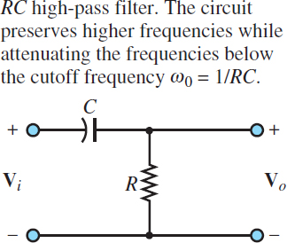
Figure 3 RC High-pass filter
The frequency response is defined as:
\[H (j\omega )=\frac{{{V}_{0}}}{{{V}_{i}}}(j\omega )\]
Voltage division yields:
\[{{V}_{0}}(j\omega )={{V}_{i}}(j\omega )\frac{R}{R+1/j\omega C}={{V}_{i}}(j\omega )\frac{j\omega CR}{1+j\omega CR}\begin{matrix}{} & (11) \\\end{matrix}\]
Thus, the frequency response of the filter is:
\[\frac{{{V}_{0}}}{{{V}_{i}}}(j\omega )=\frac{j\omega CR}{1+j\omega CR}\begin{matrix}{} & (12) \\\end{matrix}\]
Which can be expressed in magnitude-and-phase form by
\[\begin{align}& H (j\omega )=\frac{{{V}_{0}}}{{{V}_{i}}}(j\omega )=\frac{j\omega CR}{1+j\omega CR}=\frac{\omega CR{{e}^{j\pi /2}}}{\sqrt{1+{{(\omega CR)}^{2}}}{{e}^{j\arctan (\omega CR/1)}}} \\& =\frac{\omega CR}{\sqrt{1+{{(\omega CR)}^{2}}}}.{{e}^{j\left[ \pi /2-\arctan (\omega CR) \right]}} \\\end{align}\]
Or
\[\begin{matrix}H (j\omega )=\left| H \right|{{e}^{j\angle H }} & {} & \left( 13 \right) \\\end{matrix}\]
with
\[\begin{matrix}\left| H (j\omega ) \right|=\frac{\omega CR}{\sqrt{1+{{(\omega CR)}^{2}}}} & {} & {} \\{} & {} & (14) \\\angle H (j\omega )={{90}^{o}}-\arctan (\omega CR) & {} & {} \\\end{matrix}\]
You can verify by inspection that the amplitude response of the high-pass filter will be zero at ω = 0 and will asymptotically approach 1 as ω approaches infinity while the phase shift is π/2 at ω = 0 and tends to zero for increasing ω.
Amplitude and phase response curves for the high-pass filter are shown in Figure 4. These plots have been normalized to have the filter cutoff frequency ω0 = 1 rad/s. Note that, once again, it is possible to define a cutoff frequency at ω0 = 1/RC in the same way as was done for the low-pass filter.
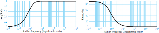
Figure 4 Frequency response of an RC high-pass filter
