Frequency response plots of linear systems are often displayed in the form of logarithmic plots, called Bode plots after the mathematician Hendrik W. Bode, where the horizontal axis represents frequency on a logarithmic scale (base 10) and the vertical axis represents either the amplitude or phase of the frequency response function. In Bode plots the amplitude is expressed in units of decibels (dB), where
\[\begin{matrix}{{\left| \frac{{{A}_{0}}}{{{A}_{i}}} \right|}_{dB}}=20{{\log }_{10}}\left| \frac{{{A}_{0}}}{{{A}_{i}}} \right|=20{{\log }_{10}}\left| \frac{{{A}_{0}}}{{{A}_{i}}} \right| & {} & (1) \\\end{matrix}\]
While logarithmic plots may at first seem a daunting complication, they have two significant advantages:
1. The product of terms in a frequency response function becomes a sum of terms because log(ab/c) = log(a) + log(b) − log(c). The advantage here is that Bode (logarithmic) plots can be constructed from the sum of individual plots of individual terms. Moreover, there are only four distinct types of terms present in any frequency response function:
a. A constant K.
b. Poles or zeros “at the origin”(jω).
c. Simple poles or zeros (1 + jωτ) or (1 + jω/ωo).
d. Quadratic poles or zeros [1+ jωτ +(jω/ωn)2].
2. The individual Bode plots of these four distinct terms are all well approximated by linear segments, which are readily summed to form the overall Bode plot of more complicated frequency response functions.
RC Low-Pass Filter Bode Plots
Consider the RC low-pass filter. The frequency response function is:
\[\frac{{{V}_{0}}}{{{V}_{i}}}(j\omega )=\frac{1}{1+j\omega /{{\omega }_{0}}}=\frac{1}{\sqrt{1+{{(\omega /{{\omega }_{0}})}^{2}}}}\angle -{{\tan }^{-1}}\left( \frac{\omega }{{{\omega }_{0}}} \right)\begin{matrix}{} & (2) \\\end{matrix}\]
where the circuit time constant is τ = RC = 1/ω0 and ω0 is the cutoff, or half- power, frequency of the filter. This frequency response function has a constant of value K = 1 and a simple pole with cutoff frequency ω0 = 1/τ = 1/RC.
Figure 1 shows the Bode magnitude and phase plots for the filter.
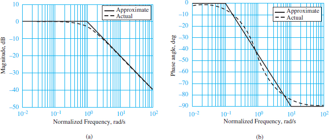
Figure 1 Bode plots for a low-pass RC filter; the frequency variable is normalized to ω/ω0. (a) Magnitude response; (b) phase angle response
The normalized frequency on the horizontal axis is ωτ. The magnitude plot is obtained from the logarithmic form of the absolute value of the frequency response function.
\[{{\left| \frac{{{V}_{0}}}{{{V}_{i}}} \right|}_{dB}}=20{{\log }_{10}}\frac{\left| K \right|}{\left| 1+j\omega \tau \right|}=20{{\log }_{10}}\frac{\left| K \right|}{\left| 1+j\omega /{{\omega }_{0}} \right|}\begin{matrix}{} & (3) \\\end{matrix}\]
When ω ≪ ω0, the imaginary part of the simple pole is much smaller than its real part, such that |1 + jω/ω0| ≈ 1. Then:
\[\begin{matrix}{{\left| \frac{{{V}_{0}}}{{{V}_{i}}} \right|}_{dB}}\approx 20{{\log }_{10}}K-20{{\log }_{10}}1=20{{\log }_{10}}K & (dB) & (4) \\\end{matrix}\]
Thus, at very low frequencies (ω ≪ ω0), equation 3 is well approximated by a straight line of zero slope, which is the low-frequency asymptote of the Bode magnitude plot.
When ω ≫ ω0, the imaginary part of the simple pole is much larger than its real part, such that |1 + jω/ω0| ≈ | jω/ω0| = (ω/ω0). Then:
\[\begin{matrix}{{\left| \frac{{{V}_{0}}}{{{V}_{i}}} \right|}_{dB}}\approx 20{{\log }_{10}}K-20{{\log }_{10}}\frac{\omega }{{{\omega }_{0}}} & {} & {} \\{} & {} & (5) \\\approx 20{{\log }_{10}}K-20{{\log }_{10}}\omega +20{{\log }_{10}}{{\omega }_{0}} & {} & {} \\\end{matrix}\]
Thus, at very high frequencies (ω ≫ ω0), equation 3 is well approximated by a straight line of −20 dB per decade slope that intercepts the log ω axis at log ω0. This line is the high-frequency asymptote of the Bode magnitude plot. A decade represents a factor of 10 change in frequency. Thus, a one decade increase in ω is equivalent to a unity change in log ω.
Finally, when ω = ω0, the real and imaginary parts of the simple pole are equal, such that |1 + jω/ω0| = |1 + j| = $\sqrt{2}$ . Then equation 3 becomes:
\[20{{\log }_{10}}\frac{\left| K \right|}{\left| 1+j\omega /{{\omega }_{0}} \right|}=20{{\log }_{10}}K-20\log \sqrt{2}=20{{\log }_{10}}K-3dB\begin{matrix}{} & (6) \\\end{matrix}\]
Thus, the Bode magnitude plot of a first-order low-pass filter is approximated by two straight lines intersecting at ω0. Figure 1(a) clearly shows the approximation. The actual Bode magnitude plot is 3 dB lower than the approximate plot at ω = ωo, the cutoff frequency.
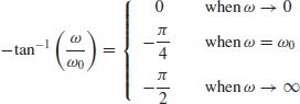
The phase angle of the frequency response function $\angle \left( \frac{{{V}_{o}}}{{{V}_{i}}} \right)=-{{\tan }^{-1}}\left( \frac{\omega }{{{\omega }_{o}}} \right)$ has the following properties:
As a first approximation, the phase angle can be represented by three straight lines:
- For ω < 0.1ωo, ∠ (Vo/Vi) ≈ 0.
- For 0.1 ωo and 10ωo, ∠ (Vo/Vi) ≈ – (π/4) log (10ω/ωo).
- For ω > 10ωo, ∠ (Vo/Vi) ≈ –pi/2.
These straight-line approximations are illustrated in Figure 1(b).
Table 1 lists the differences between the actual and approximate Bode magnitude and phase plots. Note that the maximum difference in magnitude is 3 dB at the cutoff frequency; thus, the cutoff is often called the 3-dB frequency or the half-power frequency.
Table 1 Correction factors for asymptotic approximation of first-order filter
| ω/ω0 | Magnitude response error, (dB) | Phase response error (deg) |
| 0.1 | 0 | −5.7 |
| 0.5 | −1 | 4.9 |
| 1 | −3 | 0 |
| 2 | −1 | −4.9 |
| 10 | 0 | +5.7 |
RC High-Pass Filter Bode Plots
The case of an RC high-pass filter is analyzed in the same manner as was done for the RC low-pass filter. The frequency response function is:
\[\begin{matrix}\frac{{{V}_{0}}}{{{V}_{0}}}=\frac{j\omega CR}{1+j\omega CR}=\frac{j(\omega /{{\omega }_{0}})}{1+j(\omega /{{\omega }_{0}})} & {} & {} \\=\frac{(\omega /{{\omega }_{0}})\angle (\pi /2)}{\sqrt{1+{{(\omega /{{\omega }_{0}})}^{2}}}\angle \arctan (\omega /{{\omega }_{0}})} & {} & (7) \\=\frac{\omega /{{\omega }_{0}}}{\sqrt{1+{{(\omega /{{\omega }_{0}})}^{2}}}}\angle \left( \frac{\pi }{2}-\arctan \frac{\omega }{{{\omega }_{0}}} \right) & {} & {} \\\end{matrix}\]
Figure 2 depicts the Bode plots for equation 7, where the horizontal axis indicates the normalized frequency ω/ω0. Straight-line asymptotic approximations may again be determined easily at low and high frequencies. The results are very similar to those for the first-order low-pass filter.
For ω < ω0, the Bode magnitude approximation intercepts the origin (ω = 1) with a slope of +20 dB/decade. For ω > ω0, the Bode magnitude approximation is 0dB with zero slope.
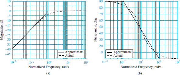
Figure 2 Bode plots for RC high-pass filter. (a) Magnitude response; (b) phase response
The straight- line approximations of the Bode phase plot are:
- For ω < 0.1ωo, ∠ (Vo/Vi) ≈ π/2.
- 2. For 0.1ωo and 10ωo, ∠ (Vo/Vi) ≈ − (π/4) log (10ω/ωo).
- For ω > 10ωo, ∠ (Vo/Vi) ≈ 0.
These straight-line approximations are illustrated in Figure 2(b).
Bode Plots of Higher-Order Filters
Bode plots of high-order systems may be obtained by combining Bode plots of factors of the higher-order frequency response function. Let, for example,
\[H (j\omega )={{H }_{1}}(j\omega ){{H }_{2}}(j\omega ){{H }_{3}}(j\omega )\begin{matrix}{} & {} & ( \\\end{matrix}8)\]
which can be expressed, in logarithmic form, as
\[{{\left| H (j\omega ) \right|}_{dB}}={{\left| {{H }_{1}}(j\omega ) \right|}_{dB}}+{{\left| {{H }_{2}}(j\omega ) \right|}_{dB}}+{{\left| {{H }_{3}}(j\omega ) \right|}_{dB}}\begin{matrix}{} & {} & ( \\\end{matrix}9)\]
And
\[\angle H (j\omega )=\angle {{H }_{1}}(j\omega )+\angle {{H }_{2}}(j\omega )+\angle {{H }_{3}}(j\omega )\begin{matrix}{} & {} & ( \\\end{matrix}10)\]
Consider as an example the frequency response function
\[H (j\omega )=\frac{j\omega +5}{(j\omega +10)(j\omega +100)}\begin{matrix}{} & {} & (11) \\\end{matrix}\]
The first step in computing the asymptotic approximation consists of factoring each term in the expression so that it appears in the form ai ( jω/ωi +1), where the frequency ωi corresponds to the appropriate 3-dB frequency, ω1, ω2, or ω3. For example, the function of equation 11 is rewritten as:
\[\begin{matrix}H (j\omega )=\frac{5(j\omega /5+1)}{10(j\omega /10+1)100(j\omega /100+1)} & {} & {} \\{} & {} & (12) \\\frac{0.005(j\omega /5+1)}{10(j\omega /10+1)100(j\omega /100+1)}=\frac{K(j\omega /{{\omega }_{1}}+1)}{(j\omega /{{\omega }_{2}}+1)(j\omega /{{\omega }_{3}}+1)} & {} & {} \\\end{matrix}\]
Equation 12 can now be expressed in logarithmic form:
\[\begin{matrix}H (j\omega ){{\left| _{dB}=\left| 0.005 \right| \right.}_{dB}}+\left| \frac{j\omega }{5}+1 \right|-\left| \frac{j\omega }{10}+1 \right|-\left| \frac{j\omega }{100}+1 \right| & {} & {} \\{} & {} & (13) \\\angle H (j\omega )=\angle 0.005+\angle \left( \frac{j\omega }{5}+1 \right)-\angle \left( \frac{j\omega }{10}+1 \right)-\angle \left( \frac{j\omega }{5}+1 \right) & {} & {} \\\end{matrix}\]
Each of the terms in the logarithmic magnitude expression can be plotted individually.
The constant corresponds to the value −46 dB, plotted in Figure 3(a) as a line of zero slope.
The numerator term, with a 3-dB frequency ω1 = 5, is expressed in the form of the first-order Bode plot of Figure 1(a), except for the fact that the slope of the line leaving the zero axis at ω1 = 5 is +20 dB/decade; each of the two denominator factors is similarly plotted as lines of slope −20 dB/decade, departing the zero axis at ω2 = 10 and ω3 = 100.
You see that the individual factors are very easy to plot by inspection once the frequency response function has been normalized in the form of equation 9.
If we now consider the phase response portion of equation 13, we recognize that the first term, the phase angle of the constant, is always zero.
The numerator first-order term, on the other hand, can be approximated, that is, by drawing a straight line starting at 0.1ω1 =0.5, with slope +π/4rad/decade (positive because this is a numerator factor) and ending at 10ω1 = 50, where the asymptote +π/2 is reached.
The two denominator terms have similar behavior, except for the fact that the slope is −π/4 and that the straight line with slope −π/4 rad/decade extends between the frequencies 0.1ω2 and 10ω2, and 0.1ω3 and 10ω3, respectively.
Figure 3 depicts the asymptotic approximations of the individual factors in equation 13, with the magnitude factors shown in Figure 3(a) and the phase factors in Figure 3(b). When all the asymptotic approximations are combined, the complete frequency response approximation is obtained.
Figure 4 depicts the results of the asymptotic Bode approximation when compared with the actual frequency response functions.
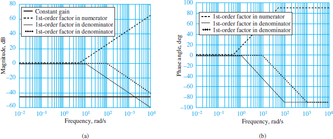
Figure 3 Bode plot approximation for a second-order frequency response function. (a) Straight-line approximation of magnitude response; (b) straight-line approximation of phase angle response
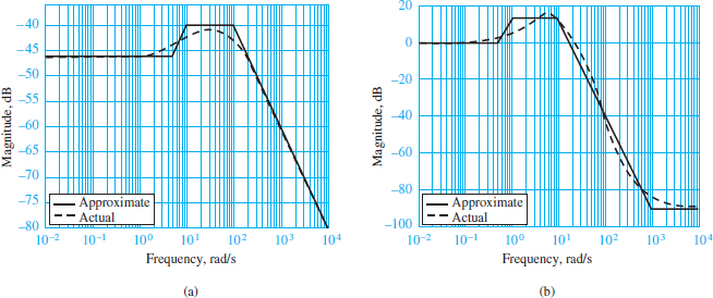
Figure 4 Comparison of Bode plot approximation with the actual frequency response function. (a) Magnitude response of second-order frequency response function; (b) phase angle response of second-order frequency response function.
You can see that once a frequency response function is factored into the appropriate form, it is relatively easy to sketch a good approximation of the Bode plot, even for higher-order frequency response functions.
Bode Plot Step by Step Guide
This section illustrates the Bode plot asymptotic approximation construction procedure. The method assumes that there are no complex conjugate factors in the response and that both the numerator and denominator can be factored into first-order terms with real roots.
1. Express the frequency response function in factored form, resulting in an expression similar to the following:
\[H\left( j\omega \right)=\frac{K\left( {j\omega }/{{{\omega }_{1}}+1}\; \right)\cdots \left( {j\omega }/{{{\omega }_{m}}+1}\; \right)}{\left( {j\omega }/{{{\omega }_{m+1}}+1}\; \right)\cdots \left( {j\omega }/{{{\omega }_{n}}+1}\; \right)}\]
2. Select the appropriate frequency range for the semi logarithmic plot, extending at least a decade below the lowest 3-dB frequency and a decade above the highest 3-dB frequency.
3. Sketch the magnitude and phase response asymptotic approximations for each of the first-order factors, using the techniques illustrated in Figures 1 to 4.
4. Add, graphically, the individual terms to obtain a composite response.
5. If desired, apply the correction factors of Table 1.
