First-order systems are important in all engineering disciplines and occur frequently in nature. Such systems are characterized by a single state variable, where the system energy is proportional to the square of the state variable. That energy is dissipated by the system such that the rate of change of the state variable is proportional to the state variable itself. The fundamental result is that the transient response of a first- order system is a decaying exponential function of time.
Ideal first-order electrical systems possess either capacitance or inductance (but not both) along with resistance and (perhaps) energy sources. Ideal first-order mechanical systems possess mass and damping (e.g., sliding or viscous friction) but no elasticity or compliance.
An ideal first-order fluid system possesses fluid capacitance and viscous dissipation, such as a hydraulic system with a liquid-filled tank and a variable orifice. Many conductive and convective thermal systems also exhibit first-order behavior.
In general, when solving transient circuit problems, it is necessary to determine three elements: (1) the steady-state response prior to a transient event, (2) the transient response immediately following the transient event, and (3) the long-term steady-state response remaining after the transient response has decayed away.
The steps involved in computing the complete response of a first-order circuit with constant sources are outlined below. The methodology is straightforward and can be mastered with only modest practice.
Circuit Simplification for t > 0
The first step to solve for the response after the transient event (t > 0) is to partition the circuit into a source network and load, with the energy storage element as the load, as shown in Figure 1. If the source network is linear, it can be replaced by its The ́venin or Norton equivalent network.
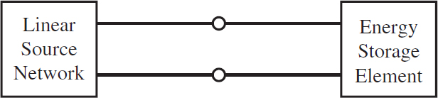
Figure 1 Generalized first-order circuit seen as a source network attached to an energy storage element as the load
Consider the case when the load is a capacitor and the source network is replaced by its Thevenin equivalent network, as shown in Figure 2.
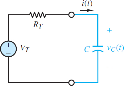
Figure 2 Generalized first-order circuit with a capacitor load and a Thevenin source
KVL can be applied around the loop to yield:
${{V}_{T}}-i{{R}_{T}}-{{v}_{C}}=0$
Of course, i = iC and for a capacitor iC = C dvC /dt. After substituting and rear-ranging the terms, the result is:
$\begin{matrix}{{R}_{T}}C\frac{d{{v}_{C}}}{dt}+{{v}_{C}}={{V}_{T}} & Capacitor\text{ }load\text{ }with\text{ }Thevenin\text{ }source & \left( 1 \right) \\\end{matrix}$
For a DC source network, the long-term steady-state solution is simply vC = VT.
Likewise, consider the case when the load is an inductor and the source network is replaced by its Norton equivalent network, as shown in Figure 3.
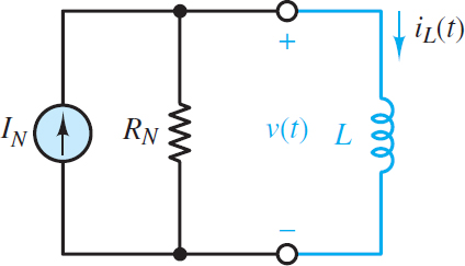
Figure 3 Generalized first-order circuit with an inductor load and a Norton source
KCL can be applied at either node to yield.
\[{{I}_{N}}-\frac{v}{{{R}_{N}}}-i=0\]
Of course, v = vL and for an inductor vL = LdiL/dt. After substituting and rearranging the terms, the result is:
$\begin{matrix}\frac{L}{{{R}_{N}}}\frac{d{{i}_{L}}}{dt}+{{i}_{L}}={{I}_{N}} & Inductor\text{ }load\text{ }with\text{ }Norton\text{ }source & \left( 2 \right) \\\end{matrix}$
For a DC source network, the long-term steady-state solution is simply iL = IN . It is also possible to use a Norton or The ́venin source when the load is a capacitor or inductor, respectively. The results can be shown to be identical to those found above by substituting the source transformation expressions VT = IN RT and RT = RN .
It is important to keep in mind that these solutions are for t > 0, that is, the transient response. It is possible that the equivalent source network seen by the load after the transient event is different from that seen by the load before the event. Equivalent network methods can be used for both domains but do not assume that the equivalent network seen by the load is unchanged by the event.
First-Order Differential Equation
Both equations 1 and 2 have the same general form:
$\begin{matrix}\tau \frac{dx\left( t \right)}{dt}+x\left( t \right)={{K}_{S}}f\left( t \right)\text{ }t\ge 0\text{ } & First-order\text{ }system\text{ }equation & \left( 3 \right) \\\end{matrix}$
Where the constants τ and KS are the time constant and the DC gain, respectively. The function f (t) is assumed equal to a constant F, which represents the contribution of one or more DC sources. With that assumption in mind, the general first-order differential equation is:
$\begin{matrix}\tau \frac{dx\left( t \right)}{dt}+x\left( t \right)={{K}_{S}}F\left( t \right) & t\ge 0 & \left( 4 \right) \\\end{matrix}$
The solution for x(t) has two parts: the transient response and the long-term steady-state response. These two parts can also be rearranged in terms of natural and forced responses. The sum of both parts is known as the complete response. One initial condition $x\left( {{0}^{+}} \right)$is needed to specify the complete response.
First-Order Transient Response
The transient response xTR is found by setting F = 0 in equation 4 such that:
$\begin{matrix}\tau \frac{d{{x}_{T}}_{R}\left( t \right)}{dt}+{{x}_{TR}}\left( t \right)=0 & {} & \left( 5 \right) \\\end{matrix}$
The solution for x is found by assuming a solution of the form:
$\begin{matrix}{{x}_{TR}}\left( t \right)=\alpha {{e}^{st}} & {} & \left( 6 \right) \\\end{matrix}$
Substitution of this assumed solution into equation 5 results in a characteristic equation:
$\begin{matrix}\tau s+1=0 & Characrteristic\_equation & \left( 7 \right) \\\end{matrix}$
The solution for s is simply:
$\begin{matrix}s=\frac{-1}{\tau } & {} & \left( 8 \right) \\\end{matrix}$
which is known as the root of the characteristic equation. Plugging in for s in equation 6 yields a decaying exponential.
$\begin{matrix} {{x}_{TR}}\left( t \right)=\alpha {{e}^{-t/\tau }} & \text{Transient Response} & \left( 9 \right) \\\end{matrix}$
The constant α in equation 9 cannot be evaluated until the complete response has been found. If the system does not have an external forcing function, the transient response is also the complete response, and the constant α is equal to the initial condition x(0+).
The amplitude of xTR (t) at t = nτ for n = 0, 1. . . 5 is shown in Figure 4. The data show that xTR has decayed by roughly 95 percent at three constants and by over 99 percent at five-time constants.
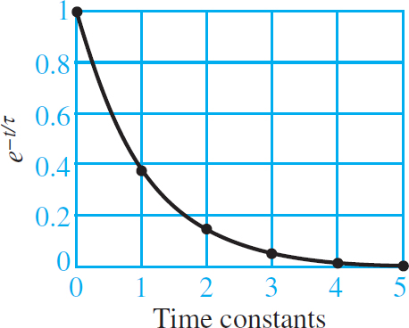
Figure 4 Normalized first-order exponential decay
Long-Term Steady-State Response
Still assuming that the first-order circuit contains only DC sources, such that f (t ) is a constant F, the long-term steady-state response of a first-order system is the solution to:
$\begin{matrix}\tau \frac{d{{x}_{ss}}\left( t \right)}{dt}={{x}_{ss}}={{K}_{s}}F & t\ge 0 & \left( 10 \right) \\\end{matrix}$
For constant F, xSS = KSF is the solution. It is a worthwhile exercise to show that this solution satisfies equation 10. Thus:
$\begin{matrix}{{x}_{ss}}\left( t \right)\equiv x\left( \infty \right)={{K}_{s}}F & \text{F=Constant} & \left( 11 \right) \\\end{matrix}$
Complete First-Order Response
The complete response is the sum of the transient and long-term steady-state responses:
$x\left( t \right)={{x}_{TR}}\left( t \right)+{{x}_{SS}}\left( t \right)=\alpha {{e}^{-t/\tau }}+x\left( \infty \right)=\alpha {{e}^{-t/\tau }}+KsF\begin{matrix}{} & t\ge 0 & \left( 12 \right) \\\end{matrix}$
Apply the one initial condition x(0+) to solve for the unknown constant α:
$\begin{matrix}x\left( {{0}^{+}} \right)=\alpha +x\left( \infty \right) & {} & {} \\{} & {} & \left( 13 \right) \\\alpha =x\left( {{0}^{+}} \right)-x\left( \infty \right) & {} & {} \\\end{matrix}$
Substitute for α in equation 12 to find the complete response:
$x\left( t \right)=\left[ x\left( {{0}^{+}} \right)-x\left( \infty \right) \right]{{e}^{-t/\tau }}+x\left( \infty \right)\begin{matrix}{} & t\ge 0 & \left( 14 \right) \\\end{matrix}$
